Special code features

The GADGET-4 code contains a number of modules that take the form of extensions of the code for specific science applications or common postprocessing tasks. Examples include merger-tree creation, lightcone outputs, or power spectrum measurements. Here we briefly describe the usage of the most important of these modules in GADGET-4.

Initial conditions

GADGET-4 contains a built-in initial conditions generator for cosmological simulations (based on the N-GenIC code), which supports both DM-only and DM plus gas simulations. Only cubical periodic boxes are supported at this point. Once the IC-module is compiled in (by setting NGENIC in the configuration), the code will create initial conditions upon regular start-up and then immediately start a simulation based on them. It is also possible to instruct the code to only create the ICs, store them in a file and then end, which is accomplished by launching the code with restartflag 6.

The NGENIC option needs to be set to the size of the FFTs used in the initial conditions creation, and the meaning of the other code parameters that are required for describing the initial conditions is described in detail in the relevant section of this guide.

Merger trees

The merger tree construction follows the concepts introduced in the paper Springel et al. (2005), http://adsabs.harvard.edu/abs/2005Natur.435..629S. It is a tree for subhalos identified within FOF groups, i.e. it requires group finding carried out with FOF, and SUBFIND or SUBFINF_HBT, and hence these options need to be enabled when MERGERTREE is set. The schematic organisation of the merger tree that is constructed is depicted in the following sketch:

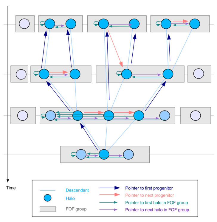
At each output time, FOF groups are identified which contain one or several (sub)halos, and the merger tree connects these halos. The FOF groups play no direct role for the tree, except that the largest halo in a given FOF group is singled out as main subhalo in the group. To organize the tree(s), a number of pointers for each subhalo need to be defined.

Each halo must know its descendant in the subsequent group catalogue at later time, and the most important step in the merger tree construction is determining this link. This can be accomplished in two ways with GADGET-4. Either one enables MERGERTREE while a simulation is run. Then for each new snapshot that is produced, the descendant pointers for the previous group catalogue are computed as well and accumulated in the output directory. The results will be written in special files called sub_desc_XXX. In essence, these provide the glue between two subsequent group catalogues. One advantage of doing this on the fly is that this allows merger tree constructions without ever having to output the particle data itself.

Alternatively, one also create these files in postprocessing for a simulation that was run without the MERGERTREE option. This however requires that snapshot files are available, or at the very least, that particle IDs have been included in the group catalogue output. The process of creating these link files can be accomplished with restartflag 7, which does this for the given snapshot number and the previous output. This has to be repeated for all snapshots except the first one (i.e. one starts at output number 1 until the last one) that should be part of the merger tree.

Finally, one can ask GADGET-4 to isolate individual trees and to arrange the corresponding subhalos in a format that allows easy processing of the trees, for example, in a semi-analytic code for galaxy formation. This process also computes the other links shown in the above sketch. To this end, one starts GADGET-4 with restartflag 8, and provides the last snapshot number as additional argument. GADGET-4 will then process all the group catalogue data and the descendant link files, and determine a new set of tree-files. The algorithms are written such that they are fully parallel and should be able to process extremely large simulations, with very large group catalogues and tree sets. The tree files will normally be split up over many files in this case, and the placing of a tree into any of these files is randomized in order to balance them roughly in size, which simplifies later processing. In order to quickly look-up based, based on a given subhalo number from one of the timeslices, in which tree this subhalo is found, corresponding pointers are added to the group catalogues as well.

Lightcone output

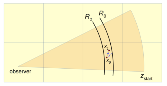
One new feature in GADGET-4 is the ability to output continuous light cones, i.e. particles are stored at the position and velocity at the moment the backwards lightcone passes over them. This is illustrated in the following sketch, which shows how the code determines an interpolated particle coordinate x' in between two endpoints of the timestepping procedure.

This option is activated with the LIGHTCONE switch, and needs to be active while the simulation is run. In this case, additional particle outputs are created, which have a structure similar to snapshot files, except that the velocities are stored directly as peculiar velocities.

While it is possible also here to use the file format 1 or 2, it is highly recommended to not bother with this but rather use HDF5 throughout for such more complicated output. This is the only sensible way to not get caught up in struggles to parse the (possibly frequently varying) binary file format.

Power spectra

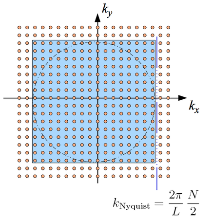
The GADGET-4 code can also be used to measure matter power spectra with a high dynamic range through the "folding technique", described in more detail in Springel et al. (2018) http://adsabs.harvard.edu/abs/2017arXiv170703397S. In essence, three power spectra are measured in each case, one for the unmodified periodic box, yielding a conventional measurement that extends up to close to the Nyquist frequency of the employed Fourier mesh (which is set by PMGRID ). The other two are extensions to smaller scales by imposing periodicity on some inter division of the box, with the box folded on top of itself. The default value for this folding factor is POWERSPEC_FOLDFAC=16 but this value can be modified if desired by overriding it with a configuration option.

The measured power spectra are outputted in a finely binned fashion in k-space as ASCII files. This data can be easily rebinned by band-averaging to any desired coarser binning (which then also reduces the statistical error for each bin), which is a task relegated to a plotting script. This can then also be used to combine the coarse and fine measurements into a single plot, and to do a shot-noise subtraction if desired. The shot-noise, allowing for variable particle masses if present, is also measured and output to the file. Example plotting scripts to parse the powerspectrum are provided in the code distribution.

There are two ways to measure the power spectra. This can either be done on the fly whenever a snapshot file is produced, by means of the POWERSPEC_ON_OUTPUT option. Or one can compute a power spectrum in postprocessing by applying the code with restartflag 4 to any of the snapshot numbers. In both cases, power spectra are measured both for the full particle distribution, and for every particle type that is present.

I/O bandwidth test

Another small feature of GADGET-4 is a stress test for the I/O subsystem of the target compute cluster. This is meant to get some information about the available I/O bandwidth for parallel write operations, and in particular, to find out whether MaxFilesWithConcurrentIO should be made smaller than the number of MPI-ranks for a specific setup to avoid that too many files being written at the same time, because this can be counter-productive in terms of throughput or cause a too high load on the I/O subsystem that inconveniences other users or jobs.

To this end, GADGET-4 can be started with the restartflag 9 option, using the same number of MPI ranks that is intended for a relevant production run. The code will then not actually carry out a simulation but instead carry out a number of systematic write tests. The tests are repeated for different settings of MaxFilesWithConcurrentIO , starting at the number of MPI ranks, and then halving this number until it drops below unity. For each of the tests, each MPI-rank tries to write 10 MB of data to files stored in the output directory (these are again deleted after the test automatically). The code then reports the effective I/O bandwidth reached for the different settings of MaxFilesWithConcurrentIO, and the results should inform about which setting is reasonable. In particular, in a regime where the I/O bandwidth only very weakly increases (i.e. strongly sub-linearly) with MaxFilesWithConcurrentIO, it will usually be better to go with a lower value where such linearity is still approximately seen to retain some responsiveness of the filesystem when GADGET-4 does parallel I/O.