Analysis scripts and Examples
On this page, we go through some examples of how to load and analyse Auriga data using some lightweight Python code, which we have made available at this bitbucket repository. These scripts are intended to be simple and flexible in order to provide a starting point that the user can build on and adapt to their specific goals.
We provide a few examples below to illustrate how these scripts can be used to analyse the data, including:
- Read snapshot data for a single particle type;
- Read the subhalo catalogues and fields;
- Center on the main galaxy and select particles;
- Converting stellar particle formation times to lookback times;
- Read and navigate the merger tree data to retrieve evolutionary histories of subhalos;
- Use the supplementary accreted star particle data to select particles from specific progenitors;
- Combine this additional information with the snapshot and merger tree data.
Snapshots & (Sub)halo catalogues
Plotting the star formation history of the main galaxy
After downloading snapshot data from the download page, start up the python interface or create a python script and import the scripts:
import auriga_public as apand then define the path to the output directory storing the data:
path='/path/to/output/directory/'For plotting the star formation history, we need only load PartType4 of the final redshift zero snapshot, which in this
case is snapshot number 127. We will also load only the following fields:
loadlist=['Coordinates', 'GFM_StellarFormationTime', 'GFM_InitialMass']which we need in order to make spatial cuts on stars (to select those confined to the galaxy), and to get their ages and initial masses.
We then create an snapshot object via
snapobj = ap.snapshot.load_snapshot(127, 4, loadlist=loadlist, snappath=path)This object contains the particle information for all star particles and wind particles thoughout the entire simulation volume, so we need to first select the particles in the main galaxy, inside say, 10 percent of the critical radius for closure. We therefore first need to retrieve the coordinates and radius of the main halo from the subhalo catalogue by creating a subhalo object:
loadlist=['SubhaloPos', 'Group_R_Crit200']
subobj = subhalos.subfind(127, directory=path, loadlist=loadlist)
We can then centre the coordinates on the main halo
snapobj = ap.util.CentreOnHalo(snapobj, subobj.data['SubhaloPos'][0])and then select only star particles within a sphere of our chosen radius
snapobj = util.apply_mask(snapobj, stars=True,
        radialcut=0.1*subobj.data['Group_R_Crit200'][0])
Finally, since the 'GFM_StellarFormationTime' is in units of scale factor, we can convert it to lookback
time under the assumption of a flat Universe with the following helper function:
ages = ap.util.GetLookbackTimeFromScaleFactor_Flat(snapobj.data['GFM_StellarFormationTime'], snapobj.hubbleparam, snapobj.omega0, snapobj.omegalambda)Now we can apply the appropriate unit conversions and make a histogram of the star formation rate
plt.hist(ages, bins=40, range=[0, 14], weights=snapobj.data['GFM_InitialMass']/(14/40)*1e10/1e9)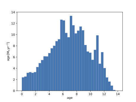
Merger Trees
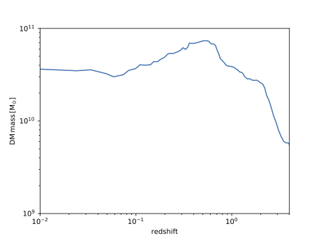
Plotting the mass evolution of a subhalo
First, load the tree for the simulation:
treeobj = ap.mergertree.load_mergertree(0, 0, 127, directory=mergertreepath)
Let us select subhalo number 1 (usually the most massive satellite) of FOF group 0 at the final snapshot, and request only the main progenitor branch of this halo
which returns the 'FirstProgenitor' indices of that object
(i.e. the main progenitor of the object at each prior snapshot) and not all the
'NextProgenitor' objects:
result = treeobj.GetObjectHistoryFromSubhaloID(1, 127, 0,
['SubhaloMassType', 'Redshift'], mainprogonly=True)
Now plot the result:
plt.plot(result['Redshift'], result['SubhaloMassType'][:,:,1]*1e10)
Accreted star particles
In this example, we demonstrate how to select star particles that were born in ex-situ in a particular subhalo, and but now belong to the main halo. This could either mean these star particles were born in a fully disrupted system, or that they have been stripped from an existing satellite galaxy. First load the accreted star particle data using the helper function
mdata = ap.util.read_starparticle_mergertree_data_hdf5(127, '/accretedstardatapath/', 'halo_6')This gives us a data object with attributes described in the data specifications page. We can get a list of all the progenitor galaxies, at the time each reached their peak stellar mass, via
first_prog = np.array(sorted(set(list(mdata['Exsitu']['PeakMassIndex']))))$ print('first_prog')
first_prog = [ -1 127 132 140 145 273 345 860 1233 1673
1930 2382 10218 10829 11280 11568 11695 11923 12907 12926
14106 14334 17599 39586 39588 41692 41911 43259 44761 45273
45512 45672 45898 47735 52804 64645 70480 70646 72024 72297
72533 74509 87696 93131 99281 102082 102097 102560 102895 102963
102988 103658 103755 103926 103966 104550 105715 105957 106642 106683
107140 108272 108455 108581 108688 108787 109362 109838 110044 110929
111064 111364 111564 117933 117958 118023 118058 118065 118168 118213
118270 118287 118451 118519 118656 118714 118775 118867 119178 119443
120081 120709 121508 121659 121809 122590 124869 125639 126335 128295
136278 148722 163753 166258 172398 209355 241501] We can count the number of star particles that are now bound to the main halo from each progenitor system, and sort in descending order
nstars_in_subhalo = np.zeros(len(first_prog))
for i, pid in zip(range(len(first_prog)),first_prog):
    nstars_in_subhalo[i] = sum( (mdata['Exsitu']['PeakMassIndex']==pid) & (mdata['Exsitu']['AccretedFlag']==0))
nsort = np.argsort(nstars_in_subhalo)[::-1]
nstars_in_subhalo = nstars_in_subhalo[nsort].astype('int')
first_prog = first_prog[nsort]
$ print('first_prog')
first_prog= [ 14334 11695 2382 39586 11923 41692 12926 99281 145 39588
1673 45273 -1 102097 860 345 14106 140 45512 108272
45672 103926 12907 108688 102895 106642 273 108455 102988 106683
10829 64645 45898 102082 118065 118058 102560 41911 93131 43259
132 119443 108787 1930 109362 103966 118023 107140 102963 121659
109838 110929 17599 127 87696 118168 111064 118775 118519 70480
241501 121809 209355 52804 119178 118714 103755 74509 120709 10218
105715 108581 1233 128295 117933 126335 117958 103658 118213 124869
118270 166258 172398 118287 118451 148722 111564 122590 120081 72533
72297 72024 70646 104550 105957 118867 118656 44761 110044 121508
111364 47735 163753 11280 11568 125639 136278]
$ print('nstars_in_subhalo')
nstars_in_subhalo= [49776 21182 21022 20657 20611 13276 12464  7198  6319  2553  1282  1264
        558   378   315   288   262   261   257   243   176   170   141    95
         94    79    79    78    48    38    35    35    34    31    24    23
         22    20    19    19    16    13    13    13    12    12    10     9
          8     8     7     7     7     7     6     6     5     4     4     4
          4     3     3     3     3     3     2     2     2     2     2     2
          2     1     1     1     1     1     1     1     1     1     1     1
          1     1     1     1     1     1     1     1     1     1     1     1
          1     1     1     1     1     0     0     0     0     0     0]
Now, we can select the particle IDs that originated from the i-th most massive contributor to the accreted stellar population.
For example, to select those from the 3rd most massive progenitor, we get the indices for which 'PeakMassIndex'=2382
and retrieve the corresponding array of 21022 'ParticleIDs'.
Combining this with other information in the accreted particle list data, such as the 'BoundFirstTime',
we may make plots such as the one below which shows the redshift 0 XYZ distribution of these star particles coloured according to the time at which they
first became unbound from their progenitor and therefore became bound to the main halo.

Here, we see that this particular satellite, whose peak logarithmic stellar mass is 8.9, has accreted over several pericentric passages, leaving shells of different extents that each comprise stars with different accretion times as defined as when they become bound to the main halo.
We can also retrieve the evolution of the progenitor above from the merger tree, via
result = treeobj.GetObjectHistoryFromMergerTreeObjectID(2382)
To see the trajectories of all the progenitor that contributed to the 5 most massive mergers in this simulation, we can find all the
'RootIndex' values associated with the 5 most massive 'PeakMassIndex'
values, and obtain from the merger tree the histories of each subhalo that ever contributed to these 5 most massive Milky Way mergers. This would produce plots like the following
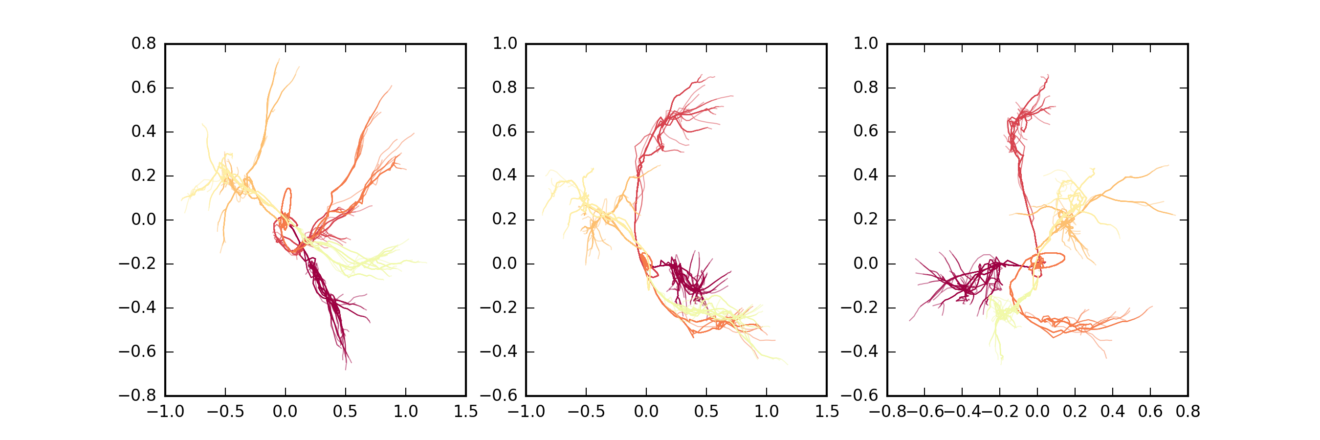
Trajectories of progenitors in the XY, XZ, YZ planes. Here, each of the 5 main mergers is made up of many smaller branches of the same colour, reflecting the earlier, smaller merger events that grow the mass of each massive progenitor until they attain their peak mass and merge with the Milky Way.
These are just a few very simple manipulations of the Auriga data products; the more detailed and interesting ones will be written by you!