|
|
|
|
|
Overview
|
|
Magneticum Pathfinder aims to follow the formation of cosmological structures in a hitherto unaccomplished level of detail by performing a set of large scale and high resolution simulations, taking into account many physical processes to allow detailed comparison to a variety of multi-wavelength observational data.
Such simulations need to incorporate a detailed description of various complex, non-gravitational, physical processes, which determine the evolution of the cosmic baryons and have an impact on their observational properties.
|
|
|
Simulations
|
Magneticum Pathfinder & Magneticum
| |
Box0 |
Box1a |
Box2b |
Box2 |
Box3 |
Box4 |
Box5 |
| [Mpc/h] |
2688 |
896 |
640 |
352 |
128 |
48 |
18 |
| mr |
2*45363 |
2*15123 |
|
2*5943 |
2*2163 |
2*813 |
|
| hr |
|
|
2*28803 |
2*15843 |
2*5763 |
2*2163 |
2*813 |
| uhr |
|
|
|
|
2*15363 |
2*5763 |
2*2163 |
| xhr |
|
|
|
|
|
2*15363 |
2*5763 |
Table 1: Number of particles used in the Magneticum Pathfinder and Magneticum simulations for the different resolution levels
mr, hr, uhr and xhr. The blue entries mark simulations which have been stopped before reaching z=0. Box2b/hr
has been stopped very close to z=0 (e.g. z~0.2). The gray entries mark future, planned simulations.
| | mdm | mgas | epsdm | epsgas | epsstars |
| mr | 1.3e10 | 2.6e9 | 10 | 10 | 5 |
| hr | 6.9e8 | 1.4e8 | 3.75 | 3.75 | 2 |
| uhr | 3.6e7 | 7.3e6 | 1.4 | 1.4 | 0.7 |
| xhr | 1.9e6 | 3.9e5 | 0.45 | 0.45 | 0.25 |
Table 2: Mass of dm and gas particles (in Msol/h) at the different resolution levels and the according softenings (in kpc/h) used.
|
|
|
|
Cosmology
Using WMAP7 cosmology taken from Komatsu et al. 2010:
- Total matter density Ω0=0.272 (16.8% baryons)
- Cosmological constant Λ0=0.728
- Hubble constant H0=70.4
- Index of the primordial power spectrum n=0.963
- Overall normalisation of the power spectrum σ8=0.809
Physics included
- cooling, star formation, winds (350 km/s) (Springel & Hernquist 2003)
- Metals, stellar population and chemical enrichment
SN-Ia, SN-II, AGB (Tornatore et al. 2003/2006)
new cooling tables (Wiersma et al. 2009)
- Black holes and AGN feedback (Springel & Di Matteo 2006, Fabjan et al. 2010)
various imrovements (Hirschmann et al. 2014), using a feedback efficiency of 0.1
- Thermal Conduction (1/20th Spitzer) (Dolag et al. 2004)
- Low viscosity scheme to track turbulence (Dolag et al. 2005)
various improvements (Beck et al. 2015)
- Higher order SPH Kernels (Dehnen & Aly 2012)
- Magnetic Fields (passive) (Dolag & Stasyszyn 2009)
|
|
|
|
|
|
Multi Cosmology Runs of Box1a/mr
| |
Ω0 |
Ωb |
σ8 |
H0 |
fb |
| C1 |
0.153 |
0.0408 |
0.614 |
66.6 |
0.267 |
| C2 |
0.189 |
0.0455 |
0.697 |
70.3 |
0.241 |
| C3 |
0.200 |
0.0415 |
0.850 |
73.0 |
0.208 |
| C4 |
0.204 |
0.0437 |
0.739 |
68.9 |
0.214 |
| C5 |
0.222 |
0.0421 |
0.793 |
67.6 |
0.190 |
| C6 |
0.232 |
0.0413 |
0.687 |
67.0 |
0.178 |
| C7 |
0.268 |
0.0449 |
0.721 |
69.9 |
0.168 |
| C8 |
0.272 |
0.0456 |
0.809 |
70.4 |
0.168 |
| C9 |
0.301 |
0.0460 |
0.824 |
70.7 |
0.153 |
| C10 |
0.304 |
0.0504 |
0.886 |
74.0 |
0.166 |
| C11 |
0.342 |
0.0462 |
0.834 |
70.8 |
0.135 |
| C12 |
0.363 |
0.0490 |
0.884 |
72.9 |
0.135 |
| C13 |
0.400 |
0.0485 |
0.650 |
67.5 |
0.121 |
| C14 |
0.406 |
0.0466 |
0.867 |
71.2 |
0.115 |
| C15 |
0.428 |
0.0492 |
0.830 |
73.2 |
0.115 |
Table 2: Different cosmological parameters used in the Box1a/mr cosmology exploration runs, where
Λ0 is always set as 1 - Ω0.
In addition, for C0 and C15 there is a non radiative run for comparison and for C8
there are simulations with increased wind velocity of 500 and 800 km/s as well as with variation of the
AGN feedback efficency to be 0.05 and 0.15, respectively.
|
|
|
|
Extra Runs
|
Dark Matter control simulations
We performed dark matter only control runs for various boxes. To avoid a different sampling of the initial density fluctuations, all these runs were done using two dark matter particle species, e.g. by treating the gas particles as dark matter only particles. Available dark matter only simulations include Box0/mr, Box1a/mr, Box2b/hr, Box2/hr, Box3/hr, Box4/uhr and Box5/xhr. There are also some dark matter only simulations for some of the multi cosmology versions of Box1a/mr. The imprint of the baryonic physics on the mass function of haloes as covered by the simulation set can be seen in the figure at the right.
|
|
ANGUS (AustraliaN GADGET-3 early Universe Simulations)
This project aims to study the role of feedback from supernovae and black holes in the evolution of the
star formation rate function (SFRF) of high redshift (z ~ 4 - 7) galaxies and consists of a set of small,
high resolution boxes. The picture on the right shows a explorational simulation of Box5/xhr
at z=2.7.
| | Box4/0.5 | Box5 | Box6 |
| [Mpc/h] | 24 | 18 | 12 |
| uhr | 2*2883 | 2*2163 | 2*1443 |
| axhr | | 2*3843 | 2*2563 |
| xhr | | 2*5763 | 2*3843 |
Table 4: Number of particles used in the ANGUS simulations.
|
|
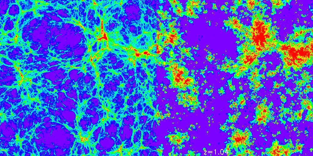
MHD simulations
Currently there are various simulations of Box3/hr as full MHD simulations available, including
simulations combining cooling and star-formation with MHD. They are probing different scenarious for the
origin of the magnetic field within the LSS. The picture on the left shows a slice through the simulation
at z=1, showing the gas density (left panel) and the magnetic field distribution (right panel), as obtained
from the magnetig field seeding from supernova events.
|
|
Post processing
|
On the fly post-processing
Similar to Saro et al. (2006), we compute the luminosities of our simulated galaxies on the fly
using the stellar population synthesis model of Bruzual & Charlot (2007) in different
spectral bands (u,V,G,r,i,z,Y,J,H,K,L,M) as well as their star-formation rate and HI content.
Following Nuzza et. al. 2010 we also take dust attenuation into account when computing the
observer frame luminosities. The attenuation is estimated from the radial dust profile,
computed from the metal and HI profile of the galaxies.
Data Management
All simulation outputs employ an algorithm which sorts the particles
among the CPUs among a space filling curve and produces an auxiliary file which
allows us to identify the sub-data volume elements of any stored property among
all particle species associated to each element of the space filling curve used.
Finally there is a super index build which allows us to identify the sub snapshots
which belongs to the different parts of the space filing curve.
This allows us to effectively collect all data associated to a given volume
in space (defined by the elements of the space filling curve it occupies)
with a minimum of reading overhead (see figure on the right).
|
|
|
|
