NIFTy Image Gallery

Wiener Filtering

1D inference without masking

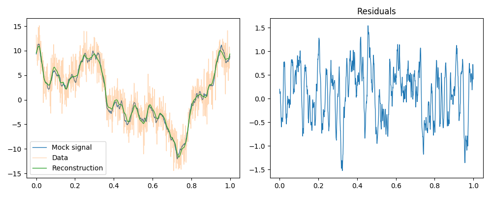
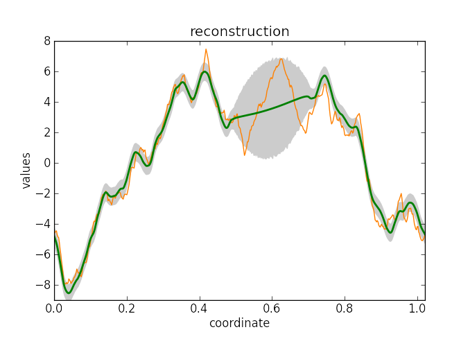
Wiener filter reconstruction of a Gaussian random signal.

Output of getting_started_1 demo, 1D mode

To reproduce, run python3 demos/getting_started_1.py 0.

1D inference with masked data

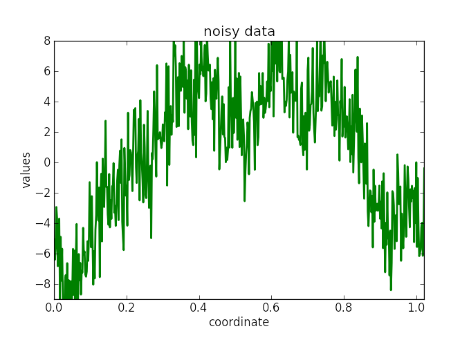
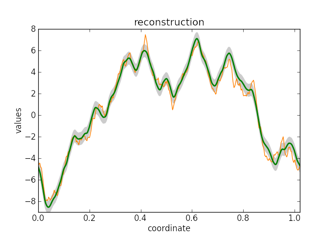
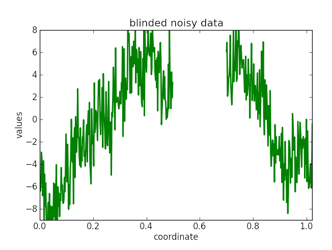
Wiener filter reconstruction results for the full and partially masked data. Shown are the original signal (orange), the reconstruction (green), and one-sigma-confidence interval (gray).

2D inference with masked data

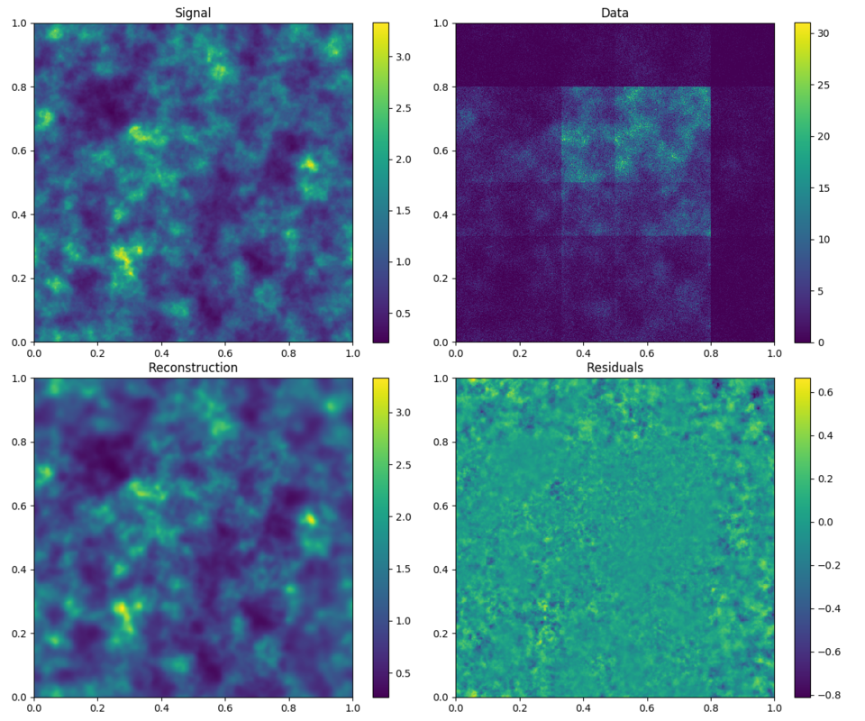
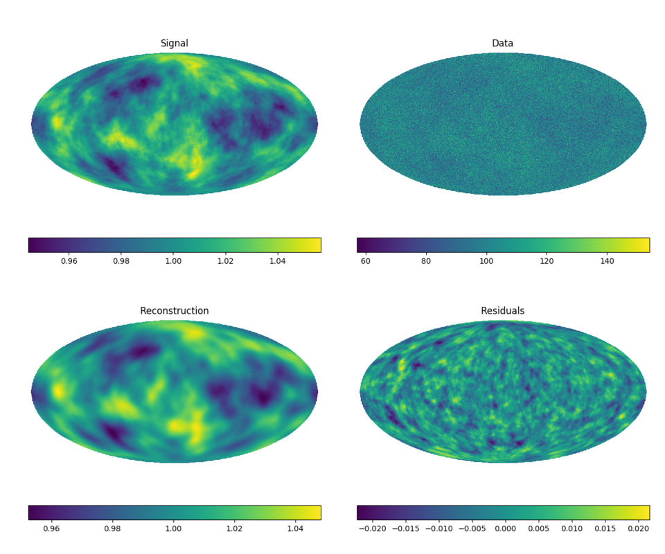
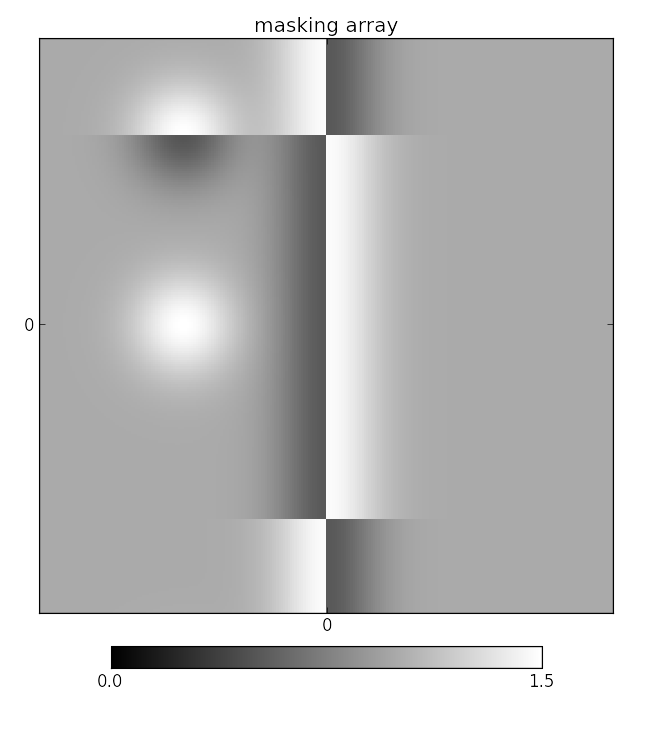
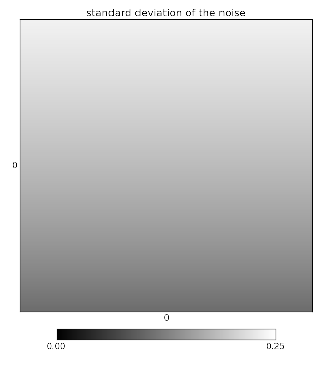
Wiener filter reconstruction of systematically and randomly masked data on a regular grid and sphere.

The same inference code is used as in ‘1D inference without masking’. Only the definitions of the signal domains and the respective masks were changed.

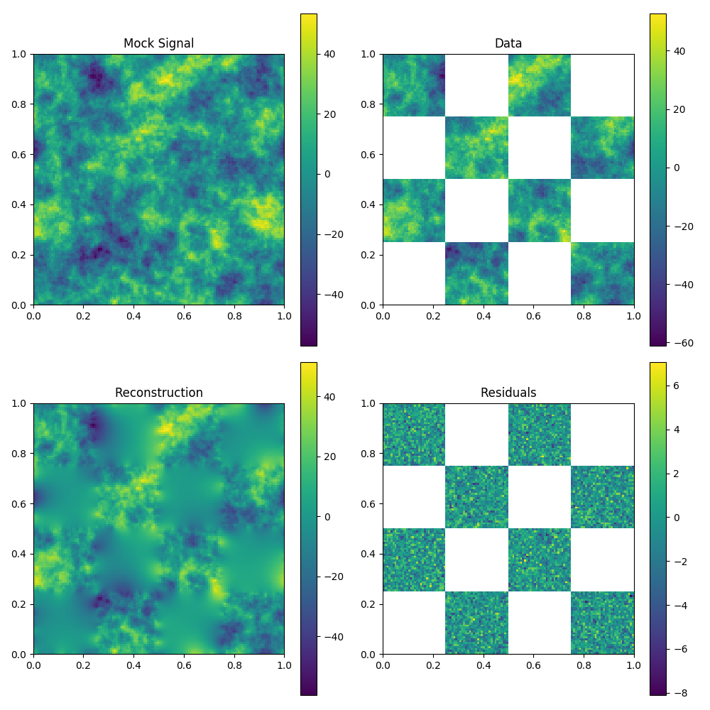
Output of getting_started_1 demo, 2D mode

To reproduce, run python3 demos/getting_started_1.py 1.

The same with a spherical domain.

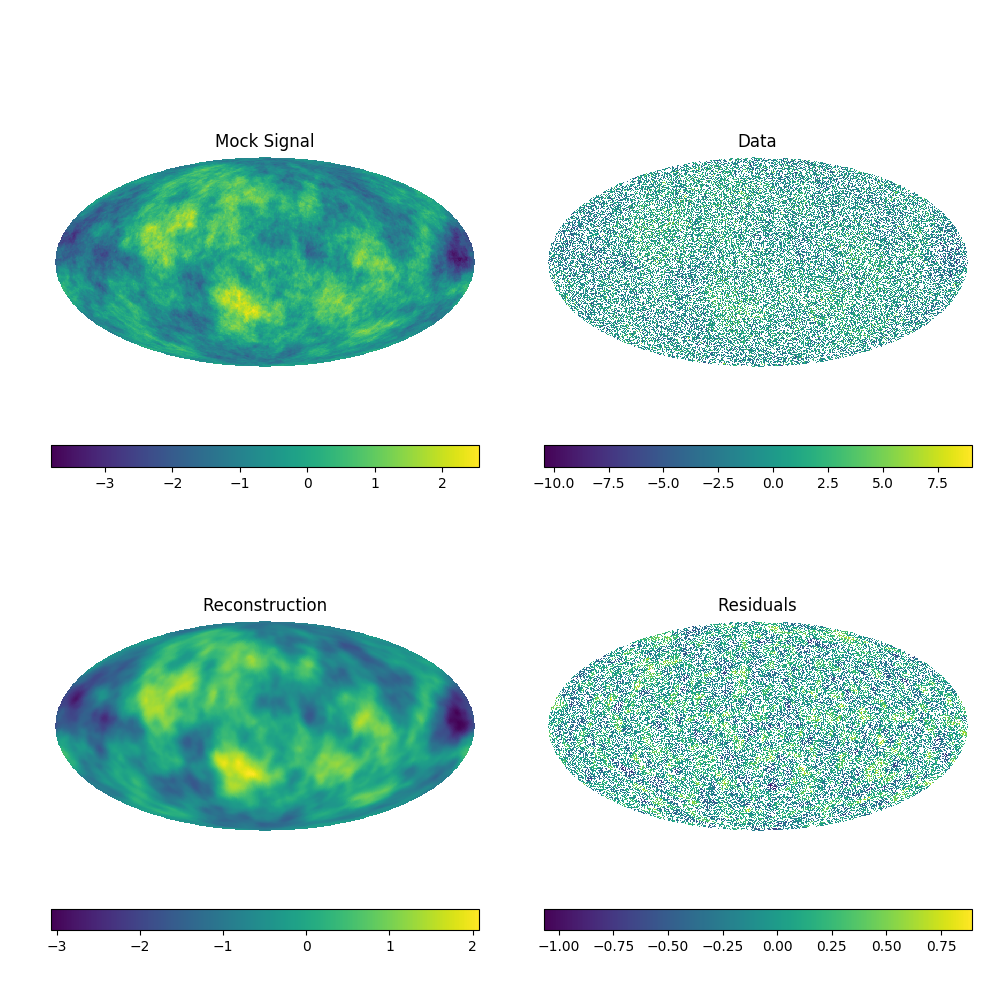
Output of getting_started_1 demo, sphere mode

To reproduce, run python3 demos/getting_started_1.py 2.

MAP analyses, Poisson statistics

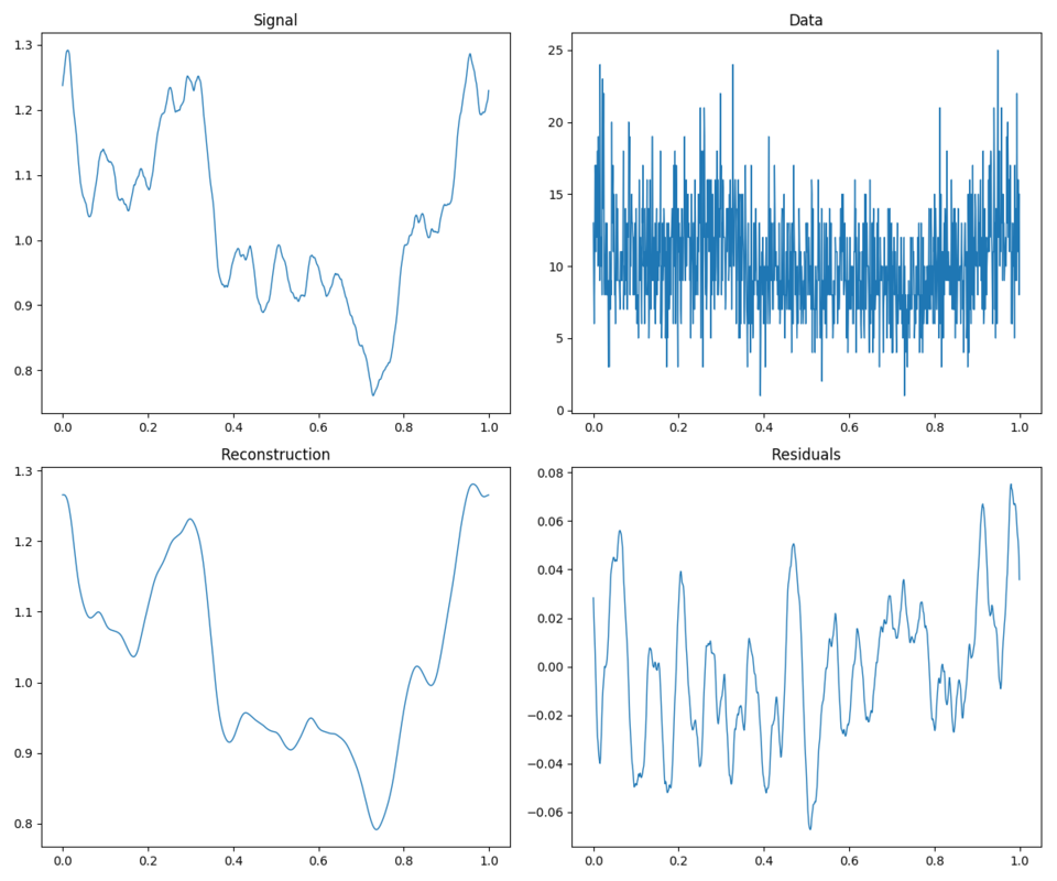
MAP reconstruction of Poissonian random signals.

All examples use the same inference code, except for the signal domain, mask and exposure definitions.

To reproduce, run python3 demos/getting_started_2.py n with n in (1, 2, 3).

Output of the getting_started_2 demo, 1D mode

2D regular grid domain.

Output of the getting_started_2 demo, 2D mode

Spherical domain.

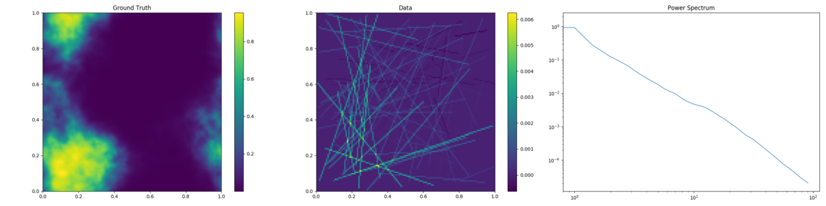
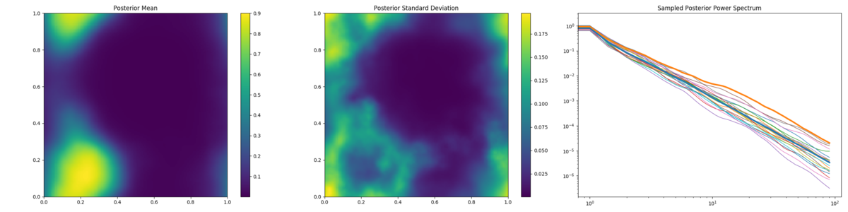
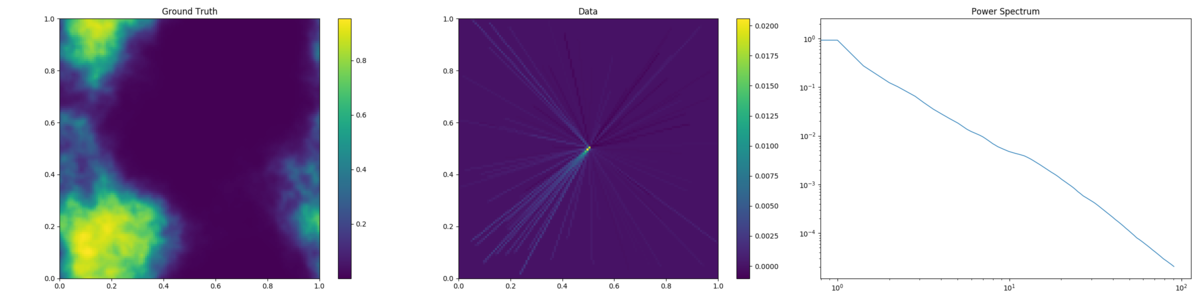
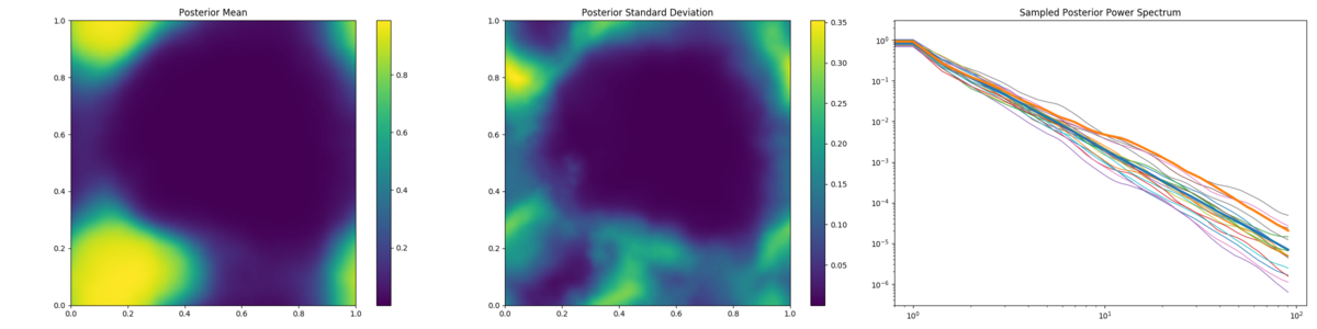
Output of the getting_started_2 demo, sphere mode

Variational Bayes inferences, Line-of-sight imaging

Variational Bayes reconstruction of LOS data, with random and radially distributed LOS.

To reproduce, run python3 demos/getting_started_3.py n with n in (1, 2).

Output of the getting_started_3 demo, random LOS, setup

Output of the getting_started_3 demo, radial LOS, setup

Transformations and Projections

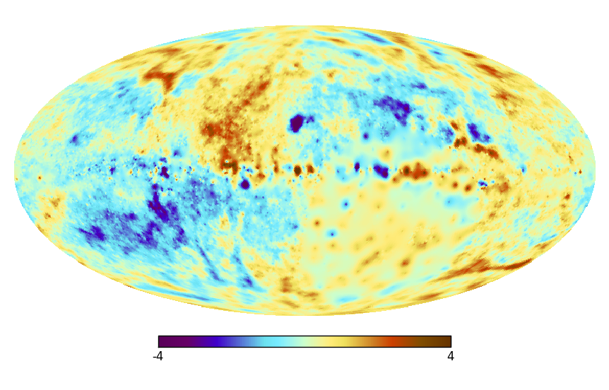
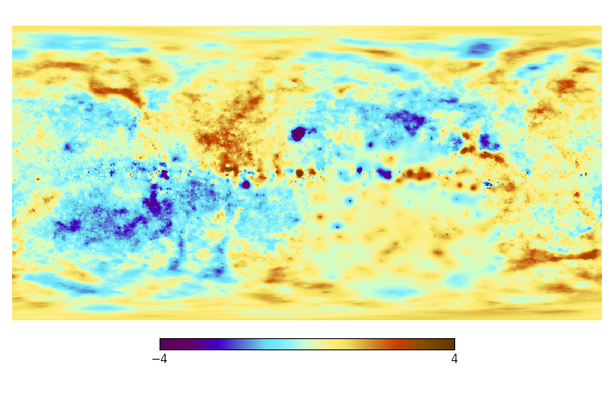
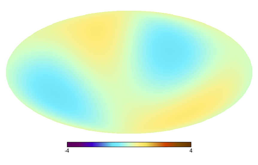
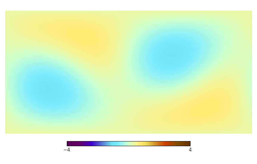
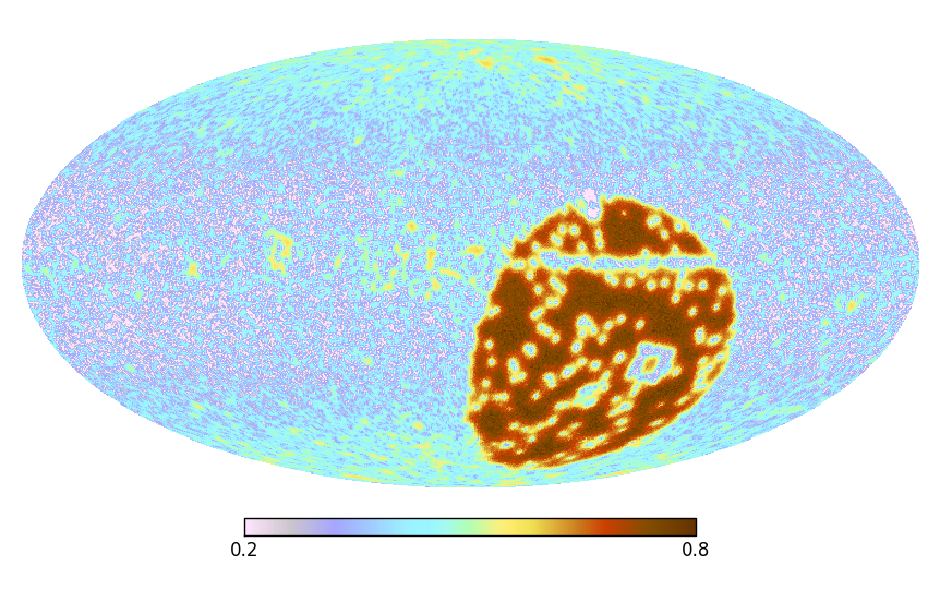
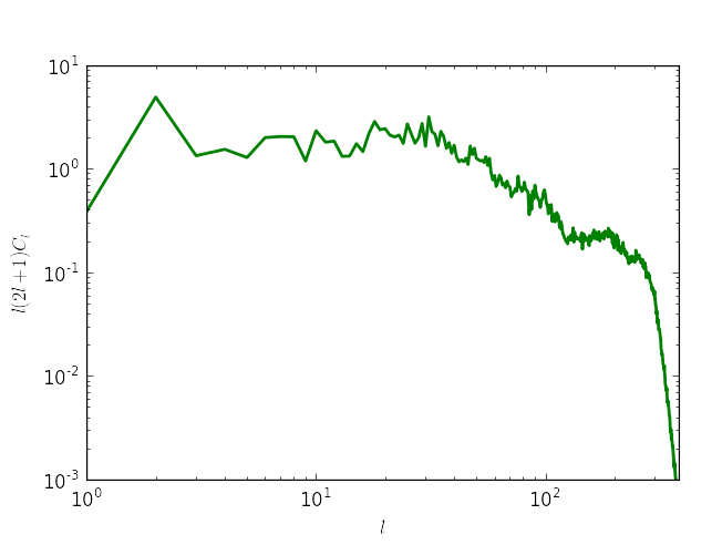
The “Faraday Map” in spherical representation on a HPSpace and a GLSpace, their quadrupole projections, the uncertainty of the map, and the angular power spectrum.

Image Reconstruction

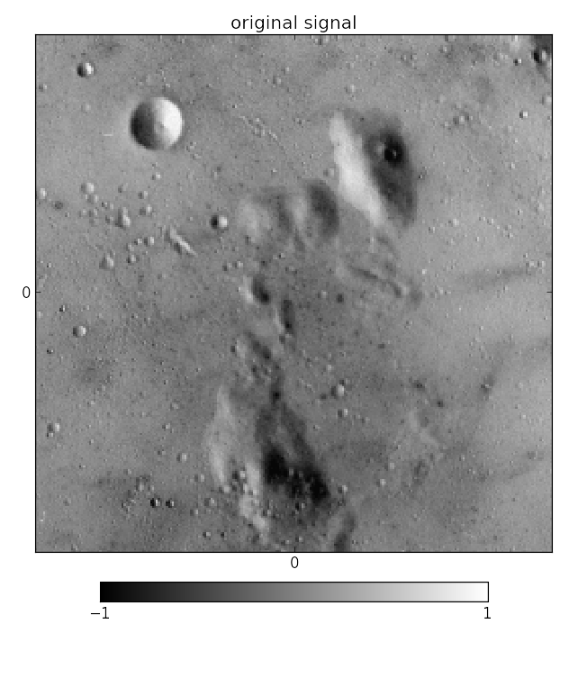
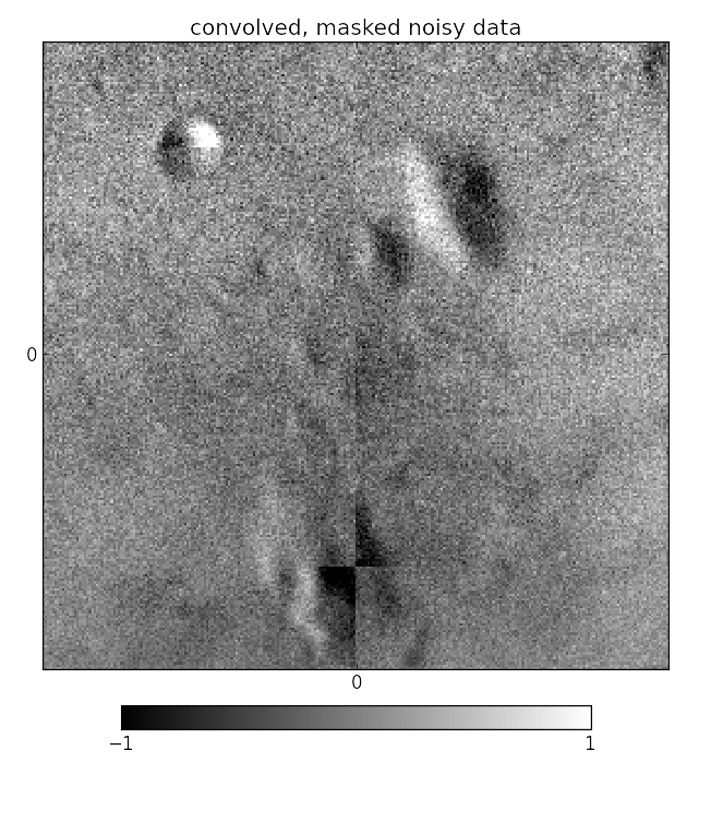
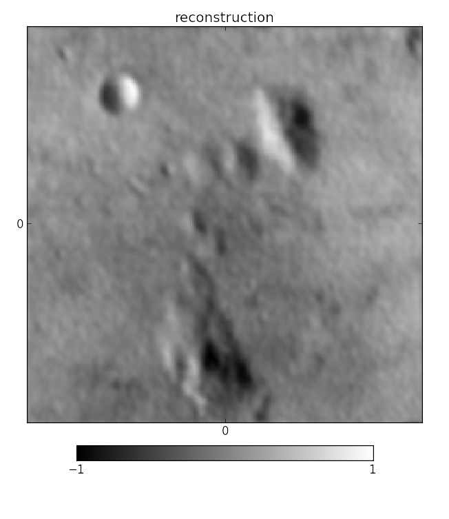
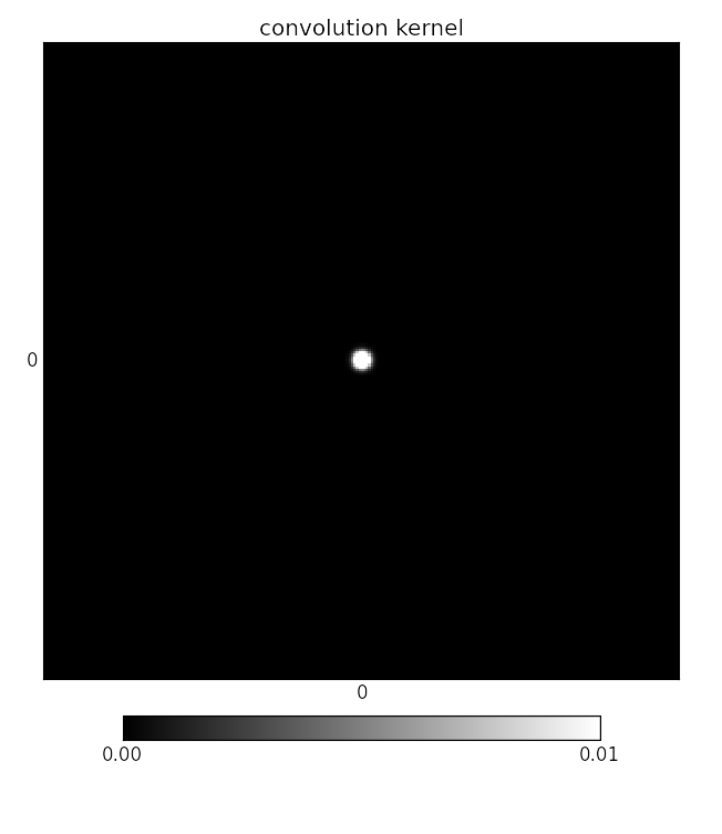
Image reconstruction of the classic “Moon Surface” image. The original image “Moon Surface” was taken from the USC-SIPI image database.