
3D Visualization: VisIVO

General information
VisIVO
(which stands for Visualization Interface for the Virtual
Observatory) is a visualization and analysis [free] software for
astrophysical data. VisIVO can handle both observational and
theoretical data (i.e. produced by numerical simulations). It can be
used both as a stand-alone application, that acts on local files, and
as an interface to the Virtual Observatory framework, from which it
can retrieve the data.
(from
http://visivo.oact.inaf.it/index.php?option=com_content&task=view&id=14&Itemid=30)
Features:
Supports multiple platforms (binaries and source)
Visualization and animation of 2D and 3D scalar and vector fields
Qualitative and quantitative data analysis
Interactive graphical user interface
Full support of the Virtual Observatory infrastructure
External links:
Supported file formats:
.msf, .zmsf; .bin, .fits, .h5, .gadget, .raw, .vot, .xml
3D Visualization: Overview
Evaluation
|
Installability |
# # # # # |
|
Functionality |
# # # # # |
|
Usability |
# # # # # |
|
Adaptability |
# # # # # |
|
Overall |
# # # # # |
VisIVO can easily be installed from
binary and requires no additional tools. Starting VisIVO you can use
the interactive interface to load in or import your data, afterwards
it is – in most cases – crucial to define the coordinates
which are not set automatically. Creating a new view (2D, 3D, plot
view or 'ortho slices') and linking one of the operations (2D, point,
surface, volume functions, plastic or table data) to it you will get
a plot which can be adjusted to your satisfaction editing the
rendering preferences, especially doing so with the Look Up Table
(LUT) can be exhausting.
VisIVO Desktop runs on the graphics
hardware of a single computer, while VisIVO Server is a grid-enabled
solution cable of using graphic cluster. Its current version is 1.5
(in July 2010), but VisIVO is still under active development; Linux
version 1.4.1-a has been tested.
Additional pros:
Instructive getting started (mainly focused on data handling)
Offers a variety of importing routines and filters (to modify VisIVO binary tables)
Modern, interactive interface
Active development
Interfaces with the Virtual Observatory
Cons:
No response during rendering process
No access to rendering option before drawing
Exhausting to use LUT (Look Up Table) editor
No crash recovery
How-to
In the following a simple introduction is given covering the installation procedure, the data file creation, its import, and a guideline towards the first plots.
How-to: Install
VisIVO can be downloaded at http://visivo.oact.inaf.it/index.php?option=com_remository&Itemid=28 for Linux, Mac OS or Windows. The source code is also available for these platforms.
To install VisIVO you may proceed in the following way:
Download the source code in a temporary directory (e.g. ~/visivoTEMP/) which can be removed after installing and change into it.
~> cd visivoTEMP/
Unpack the distribution and change into the new directory (adjusted to your version number). There is an INSTALL.README file with further information.
~/visivoTEMP>
tar -xzf visivo-setup-linux.tar.gz
~/visivoTEMP> cd
VisIVO-1.5.7.1-05052009/
Start the installation with the following command and type in the install path (e.g. ~/INSTALLDIR/) when asked.
~/visivoTEMP/VisIVO-1.5.7.1-05052009>
./install
Install dir: ~/INSTALLDIR
Visivo will be installed in the specified path in a subdirectory /VisIVO. Changing into this directory you can now run VisIVO.
~/visivoTEMP/VisIVO-1.5.7.1-05052009>
cd ~/INSTALLDIR/VisIVO
~/INSTALLDIR/VisIVO> visivo
How-to: Data
This How-to is as from now on assuming you have data of one scalar field on a structured grid.
First you have to create a BIN file simply containing all your data.
Here is a C++ code example how to do so knowing the scalars DATA[x][y][z] (of type float) and the dimensions NX, NY and NZ (all of type short int) of the grid. The data is written to a binary file (MYBINFILE.bin) ordered by increasing x, then y, and finally z.
#include
<fstream>
// Define your scalars DATA[x][y][z] and
dimensions NX, NY and NZ here!
ofstream binfile
("MYBINFILE.bin", ios::out | ios::binary);
for (int
z=0; z<N3; z++)
{ for (int y=0; y<N2;
y++)
{ for (int x=0; x<N1;
x++)
{ float
value=D[x][y][z];
binfile.write
((char*)&value, sizeof (value));
}
}
}
binfile.close();
Furthermore, you have to create a header file which contains plain text, therefor open a blank document with your editor of choice and choose one of the header types. For a detailed discussion about headers please check the VisIVO documentation.
Note: In this example for a structured grid both ways (for header or descriptor) are equivalent.
The header (MYBINFILE.bin.head) contains the data type (f for float, d for double), the number of fields (here 1), number of entries (here 64^3), the endian type (l for little, b for big endian) and the name of the field(s).
f
1
262144
l
scalars
The descriptor (MYBINFILE.bin.desc) contains a key phrase, the name of the field, number of dimensions (here 3), data type, the number of cells in each dimension (here 64), the name of the time variable, endian type (l for little, b for big endian), and the BIN file name with time id in front.
rawGridsDesc
scalars
3
Float
64
64
64
time
l
0
MYBINFILE.bin
Note: The header files are case sensitive.
How-to: Use
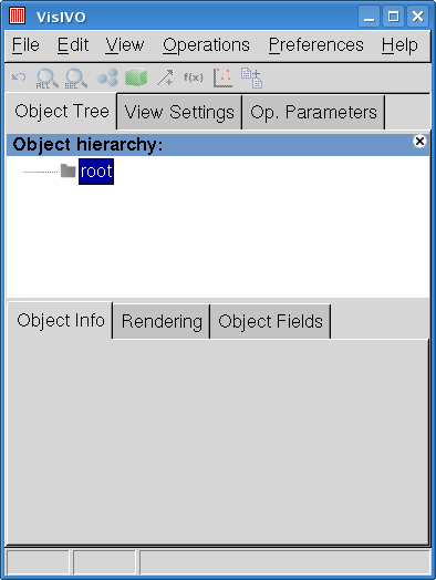
Start VisIVO and import your data.
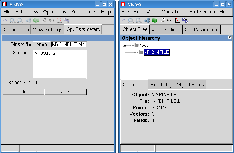
In case you use a header click File > Import > Binary, then open the binary file and select the fields.
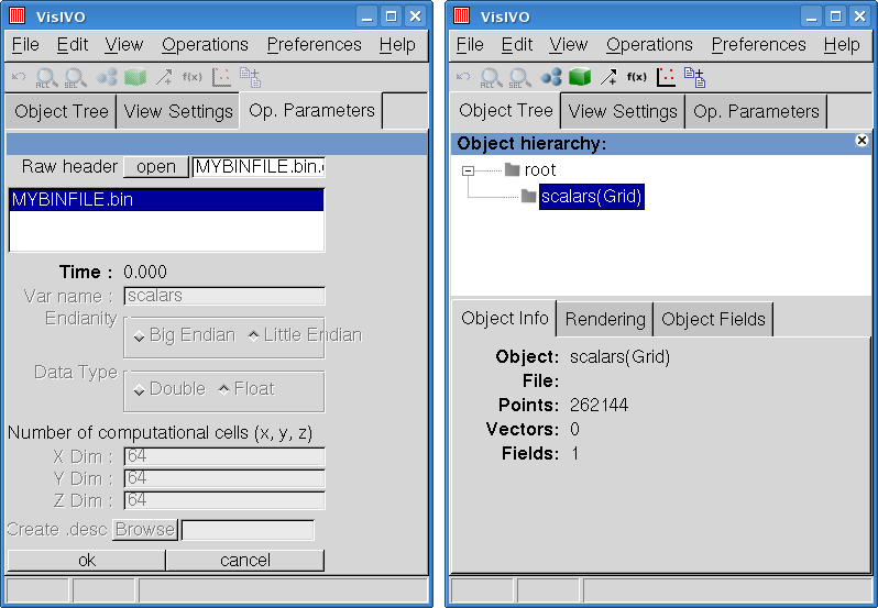
In case you use a descriptor click File > Import > Raw Grids, then open the descriptor and acknowledge.
In order to plot your table data a grid object needs to be created and adjusted.
Therefor click Operations > Table Data > Create Grid Object, select a field, set cell properties and confirm.
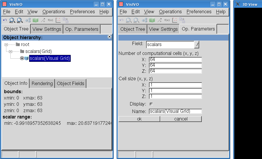
Hint: You can also use the shortcut in the menu tool bar (green cube).
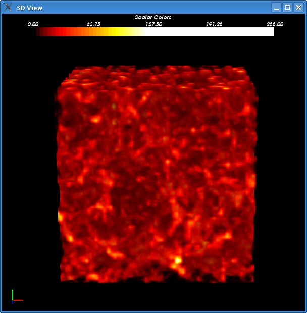
In the created 3D View you can now see the Visual Grid. The grid can be rotated keeping pressed the left mouse button, translated via middle and scaled via right mouse button.
Adjustments to the rendering can be made in the Rendering tab, there you can also modify the Look Up Table (LUT) by opening the LUT editor via double clicking.
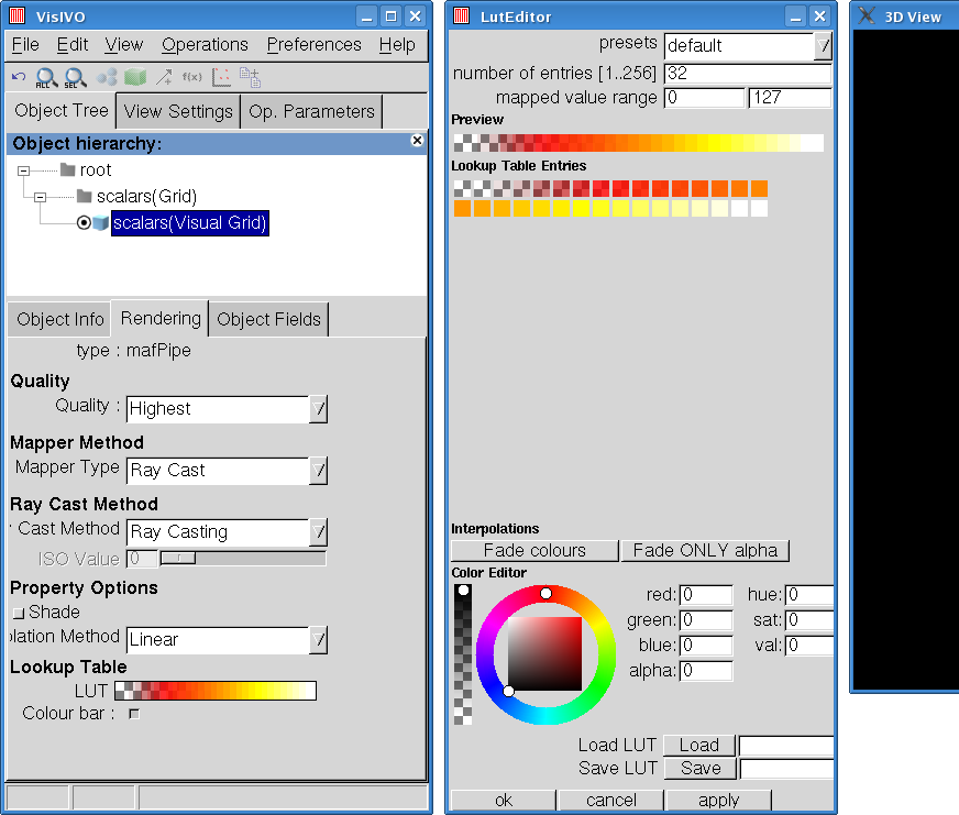
Hint: Modifying the LUT can be exhausting, therefore you may want to try MYLUT.lut.
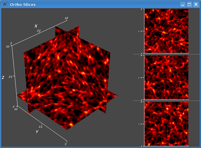
Another advantageous plot is provided by orthogonal slices through the grid object.
Add an new viewer by clicking View > Add View > Ortho Slices, then assign your data by clicking the radio button in the Object Tree tab in front of your Visual Grid. Adjustments can be made in the View Settings tab.
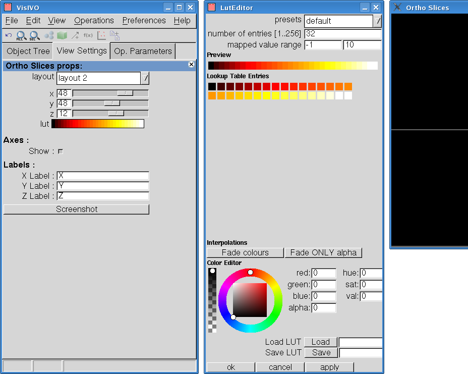
Hint: You may use the same LUT as before but correcting all alpha values to zero.
Congratulations! You can now call yourself a VisIVO user.
by
Marco Selig