3D Visualization: VAPOR

General information

VAPOR is the Visualization and Analysis Platform for Ocean, Atmosphere, and Solar Researchers – A visual data discovery environment tailored towards the specialized needs of the astro and geosciences CFD (Computational Fluid Dynamics) community, [and] a desktop solution capable of handling terascale size data sets.
(from http://www.vapor.ucar.edu/)

• Features:

  • Supports multiple platforms (binaries and source)

  • Advanced interactive 3D visualization tightly coupled with quantitative data analysis

  • Interactive graphical user interface

  • Handles multi-variate, massive time-varying data

  • Close coupling with interpretive data language (IDL)

  • Supports 3D visualization of WRF-ARW datasets

• External links:

  • VAPOR homepage

  • VAPOR documentation and download

• Supported file formats:

  .vdf;  .ncdf, .raw, .wrf

3D Visualization: Overview

Evaluation

Installability	# # # # #
Functionality	# # # # #
Usability	# # # # #
Adaptability	# # # # #

Overall

# # # # #

VAPOR can easily be installed from binary and requires no additional tools. It reads only VAPOR Data Files (VDF) and VAPOR Data Collections (VDC) respectively, but VAPOR comes along with a dozen command-line tools enabling data conversions. Once your data is loaded and set up in appropriate rendering tab (animation, viewpoint, region, 2D, probe, ISO, flow, direct volume rendering) the plot is drawn in the selected visualizer according to the edited transfer function. Due to the limited settings, apart from the transfer function, the final result will not be unalike the initial one, but quick at hand.
VAPOR uses a single computers graphics hardware (with hardware acceleration) by default. Its current version is 1.5.2 (in July 2010), but VAPOR is still under active development; Linux version 1.5.2 has been tested.

• Additional pros:

  • Quick start guide, continuative manuals

  • Graphical user interface with efficient interactivity

  • 3D rendering via 3DTexture, 3DTexture-Shader or Volumizer engines

  • User-friendly, separately savable transfer function editor

  • Active development

  • Ancillary command-line tools for data converting

• Cons:

  • Reads only its own VDF (VAPOR Data File) format

  • Less settings available

  • No opacity or color map in output

  • Tricky camera handling

  • Screenshots without image size specification

How-to

In the following a simple introduction is given covering the installation procedure, the data file conversion and a guideline towards the first plots.

How-to: Install

• VAPOR can be downloaded at http://www.vapor.ucar.edu/downloads/index.php?id=binary for Linux, Mac OS or Windows. The source code is also available for these platforms.

  Hint: Members of MPA Garching are given the alternative to use the remote visualization supported by the Rechenzentrum Garching (see http://www.rzg.mpg.de/visualisation/remote-visualization for more detailed information).

• To install VAPOR you may proceed in the following way:

  • Download the compressed binary package into a temporary directory (e.g. ~/vaporTEMP/) which can be removed after installing and change into it.

~> cd vaporTEMP/

• Extract the package and change into the new directory (adjusted to your version number).

~/vaporTEMP> tar -xf vapor-1.5.2-Linux_i386.tar.gz
~/vaporTEMP> cd vapor-1.5.2-Linux_i386/

• Start the installation script with the following command and add the installation path (e.g. ~/INSTALLDIR/vapor/). VAPOR will then be installed.

~/vaporTEMP/vapor-1.5.2-Linux_i386> ./vapor-install.csh ~/INSTALLDIR/vapor/

Note: Before starting VAPOR it is mandatory to run the configuration script each time, therefore it is advisable to place this command in your login script. Depending on your shell derivative choose the compatible command. (The first one is to be used in case of a C-shell, the second in case of Bourne-shell.)

~> source ~/INSTALLDIR/vapor/bin/vapor-setup.csh

or

~> . ~/INSTALLDIR/vapor/bin/vapor-setup.sh

• Changing into the installation directory you can now run VAPOR by executing the following command.

~/vaporTEMP/vapor-1.5.2-Linux_i386> cd ~/INSTALLDIR/vapor/bin/
~/INSTALLDIR/vapor/bin> vaporgui

How-to: Data

• VAPOR uses only its own Data Collection (VDC), but creating a raw data set and converting it in a VDF (VAPOR Data File) can be done using VAPORs command-line tools.

This How-to is as from now on assuming you have data of one scalar field on a structured grid.

• First you have to create a simple RAW file containing all your data.

  Here is a C++ code example how to do so knowing the scalars DATA[x][y][z] (of type float) and the dimensions NX, NY and NZ (all of type short int) of the grid. The data is written to a binary file (MYRAWFILE.raw) ordered by increasing x, then y, and finally z.

#include <fstream>

// Define your scalars DATA[x][y][z] and dimensions NX, NY and NZ here!

ofstream rawfile ("MYRAWFILE.raw", ios::out | ios::binary);

for (int z=0; z<N3; z++)
{  for (int y=0; y<N2; y++)
   {  for (int x=0; x<N1; x++)
      {  float value=D[x][y][z];
         rawfile.write ((char*)&value, sizeof (value));
      }
   }
}

rawfile.close();

• Secondly you run the command-line tools from the location of your RAW file (e.g. ~/MYFILES/) to create an empty VDF and then fill it with the raw data. For a detailed discussion about all tools please check the VAPOR documentation.

  • The vdfcreate tool creates a metadata file in the VDF format. You have to specify the dimensions (here 64^3), periodicity (here 1^3), the number of time steps (here 1), the name of the variable(s) and finally the new file name

~/INSTALLDIR/vapor/bin> cd ~/MYFILES/
~/MYFILES> ~/INSTALLDIR/vapor/bin/vdfcreate -dimension 64x64x64 -periodic 1:1:1 -numts 1 -vars3d scalars MYVDFFILE.vdf

• The raw2vdf tool converts your data and fills the VDF. The minimal specifications are the name of the variable(s), the target VDF and the source file.

~/MYFILES> ~/INSTALLDIR/vapor/bin/raw2vdf -varname scalars MYVDFFILE.vdf MYRAWFILE.raw

How-to: Use

• Start the VAPOR GUI.

Hint: Members of MPA Garching are given the alternative to use the remote visualization supported by the Rechenzentrum Garching (see http://www.rzg.mpg.de/visualisation/remote-visualization for more detailed information).

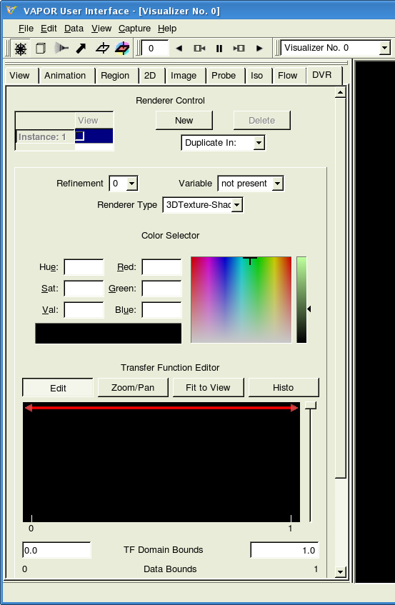
• Change to the DVR (Direct Volume Rendering) tab, load and visualize your data.

  • To load your VDF click in the menu tool bar Data > Load a Dataset into Current Session and then check View for the appropriate instance.

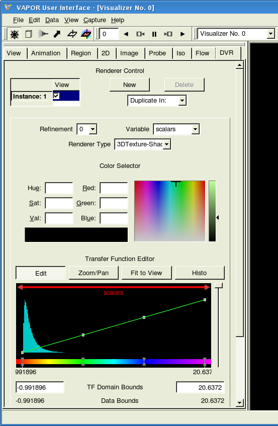
Note: The rendering type can not be change as long as the View of the instance is activated.

• The Data is plotted in the Visualizer and can be rotated keeping pressed the left mouse button, translated via middle and scaled via right mouse button.

Hint: You can alternatively modify the view in the View tab but is not advisable for unexperienced users.

• Now you can adjust the volume rendering by modifying the Transfer Function (TF) and the less available settings.

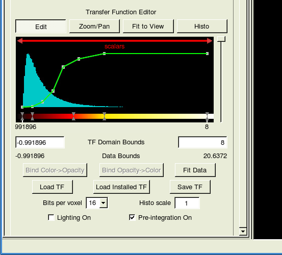
Hint: You may want to try the VAPOR Transfer Function (VTF) MYVTF.vtf.

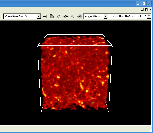
• Furthermore, you can visualize slices trough the volume in the Probe tab.

  • Check View for one of the the instances, orientate the slice and again adjust the TF.

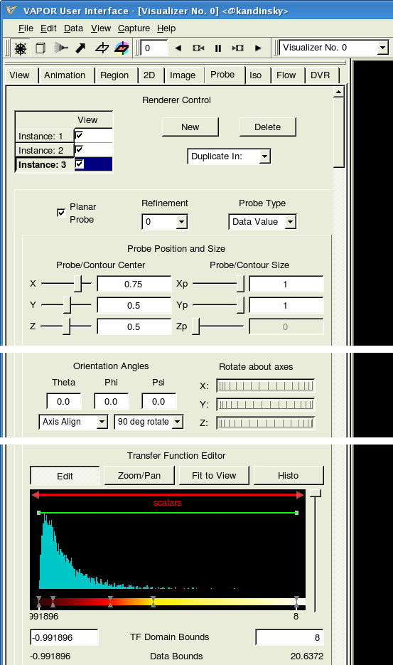
Note: Adding additional instances by clicking New, you can create as many slices as you like.

Hint: You may use the same TF as before but correcting the opacity to be always equal to one.

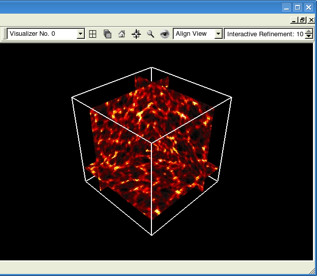
Congratulations! You can now call yourself a VAPOR user.

by Marco Selig 2010-07-19 14:36