Smac

Abstract

Smac is a map making utility for idealized observations.

Authors

This software package is currently developed by Klaus Dolag and and based on an initial version of Alessandro Gardini. It contains contribution by Bepi Tormen, Mauro Roncarelli, Elena Rasia, Matteo Maturi, Julius Donnert and Dunja Fabjan.

A description of the current implementation of the map making procedure can be found in Dolag et al. 2005.

Functionality for JobRunner

The returned fits maps contain the image in the first extension and the header gives some additional information about the parameters used for the map making, e.g. BOX_KPC contains the width of the image in units of kpc, BOX_PX holds the number of pixels and Z_KPC holds the integration length along the third dimension (in units of kpc).
The linear size of a pixel therefore is dL = BOX_KPC/BOX_PX and the area covert by a pixel is dA = (BOX_KPC/BOX_PX)^2 = 2.3245627e+45 cm^2 There is now additionally the keyword REDSHIFT indicating the redshift of the image as well as PSIZEKPC and PARCMIN indicating the pixel size in kpc and arc-min respectively.

For the JobRunner project, currently the full list of possible map making features is now available, but it has to be reminded that not all maps can be drawn from every simulations. Some of them require very special physics included. Following functionality will produce idealized observations and should be functional (click on the image to get the corresponding sample fits file):

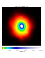
2D baryonic density map (in g/cm^2). Set:
PART_DISTR = "1 - SPH (flat 2D map)"
OUTPUT_MAP = "1 - 2D electron Density"
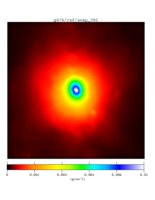g676/csf/snap_092
The hydrogen fraction of the underlying simulations are fr = 0.76, therefore the mean molecular weight is umu = 4./(5.*fr+3.) = 0.588235 and the conversion of number density of particles to number density of electrons is n2ne = (fr+0.5*(1-fr))/(2*fr+0.75*(1-fr)) = 0.517647.
The total baryonic mass within the image can be calculated as M_baryons = Sum(image*dA) = 1.3483437e+13 [M_sol].
Mass-weighted Temperature [keV]. Set:
PART_DISTR = "1 - SPH (flat 2D map)"
OUTPUT_MAP = "2 - Temperature"
OUTPUT_SUB = "0 - mass weighted"
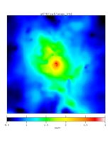g676/csf/snap_092
Emission-weighted Temperature [keV]. Set:
PART_DISTR = "1 - SPH (flat 2D map)"
OUTPUT_MAP = "2 - Temperature"
OUTPUT_SUB = "1 - emission weighted"
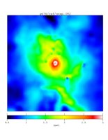g676/csf/snap_092
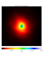
X-ray surface brightness [erg/cm^2]. Set:
PART_DISTR = "1 - SPH (flat 2D map)"
OUTPUT_MAP = "6 - X-ray SB"
OUTPUT_SUB = "0 - simple sqrt(T)"
g676/csf/snap_092
The total Luminosity within the image can be calculated as L_x = Sum(image*dA) = 5.8776952e+43 [erg/s].
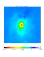
Compton Y-parameter: tSZ effect. Set:
PART_DISTR = "1 - SPH (flat 2D map)"
OUTPUT_MAP = "7 - compton y parameter (tSZ)"
OUTPUT_SUB = "1 - adimensinoal [DT/T]"
g676/csf/snap_092
Compton w-parameter: kSZ effect. Set:
PART_DISTR = "1 - SPH (flat 2D map)"
OUTPUT_MAP = "8 - kinematic SZ effect (kSZ)"
OUTPUT_SUB = "1 - adimensinoal [DT/T]"
g676/csf/snap_092
Total Mass. Set:
PART_DISTR = "3 - TSC (flat 2D map)"
OUTPUT_MAP = "101 - 2D DM density"
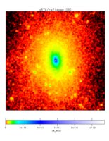g676/csf/snap_092
This calculates the total mass (dark matter + gas + stars) in every pixel in units of solar masses.
The 2D total mass density can be calculated as rho_2D = image/dA [M_sol/cm^2].
The total mass within the image can be calculated as M_tot = Sum(image) = 1.51672e+14 [M_sol].

Meaning of the parameters

IMG_XY_UNITS
Choose the units to specify the image, either arcmin or kpc. Recommended is to use kpc.

IMG_XY_SIZE
Give the size of the image. If kpc was selected as unit, useful values are of order of 1000. Note that the size is given in physical units, so be aware to choose accordingly smaller values at high redshift.

IMG_Z_SIZE
Same than IMG_XY_SIZE but describing length of the line of sight to integrate through the cluster. Use values similar to the cluster size, as the underlying simulations are limited in their proper resolved volume around the cluster (typically 3-5 R_200). Note that the value is also given in physical units, so be aware to choose accordingly smaller values at high redshift.

IMG_SIZE
Number of pixels for the image. As the background process which on the fly is calculating the image is limited in execution time on the server, do not choose large values. Typically 128 should work with all simulations.

CENTER_X,CENTER_Y,CENTER_Z
Position to center the image on, in code units. Use the aim button on the left to select a proper cluster you want to make the image from.

PROJECT
Select the axis along the projection should be performed.

OUTPUT_MAP
Select the output type of the ideal observation you want to perform.

TEMP_UNIT
Select the units for the temperature maps, either K or keV.

TEMP_CUT
Select a lower temperature of particles contribution to your observations. Can be used to exclude some of the cool cores in the simulations.

XRAY_E0,XRAY_E1
Specify the energy band for the x-ray surface brightness and the emission weighted temperature maps.

Functionality for Lightcones

The output for a light-cone has several data products, here an example of the geometry of a constructed light-cone:

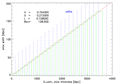
Tracing the light-cone back in time, the according slice is taken from snapshots at that epoch. The blue dashed lines mark the redshift of each slice. The green area symbolize the slice taken from each snapshot. Every of this slices has different data products (as described below), where each file will have a prefix NAME corresponding to the cosmological model used and a number, corresponding to the snapshot number it was created from.

The geometry file NAME.geometry.dat is a plain ASCII file and shows the setup of the light cone (maximum redshift, opening angle, ...) and the contribution of the individual outputs at the different redshifts. All coordinates are in [Mpc]. Most importantly, zslice indicates the redshift which correspond to each snapshot.
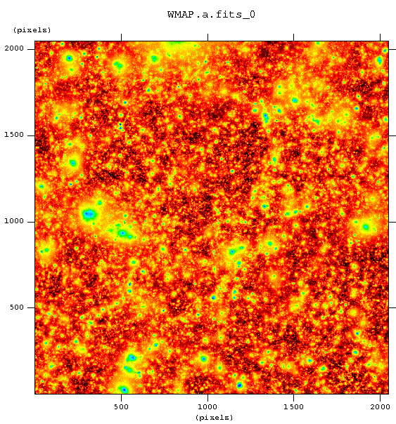
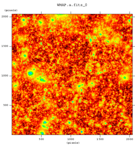
NAME.a.fits is the final map of the light-cone.
NAME.XXX.a.fits are the individual contributions of each snapshot (XXX) to the map (see NAME.geometry.dat, first column = XXX, second column = redshift).
NAME.XXX.cluster.sim.dat holds the positions of all clusters with Mvir > 1e14 within the slice of output XXX. Listed are the x,y,z coordinate (kpc/h) within the simulation box (2-4th column), their velocity (4-6th column), Mvir [Msol/h] and Rvir [kpc/h].
NAME.XXX.cluster.dat holds the same than before but giving the positions and Rvir in image coordinates (0 .. 1). Therefore the objects can be easily associated with features in the fits files.
NAME.XXX.galaxies.sim.dat Same as the one for clusters, but for all galaxies in the simulation. Instead of Mvir and Rvir the maximum circular velocity (vmax) is given, which allows to assign luminosities to the galaxies based on semi-analytic results.
NAME.XXX.galaxies.dat holds the same than before but giving the positions in image coordinates (0 .. 1). Additional the true redshift (e.g. position in the light-cone) and the observed redshift (including the peculiar velocity of the galaxies) is given, as well as the luminosities of the galaxies as predicted by the simulations in the 12 bands u V g r i z Y J H K L M are given.

Here is a small idl program showing how to convert the coordinates from the simulation into positions within the image.

Contact

Contact Klaus Dolag (kdolag@mpa-garching.mpg.de) in case of questions.