Modeling Dynamic Phases in Stellar Evolution using Multidimensional Hydrodynamics Simulations
Philipp Edelmann
Heidelberg Institute for Theoretical Studies, Germany
Motivation
- spherical symmetry
- no dynamical effects
- turbulence model with free parameters
- no enforced symmetry
- full equations of fluid dynamics
- turbulence from first principles
Low Mach Number Hydrodynamics
What?
Mach number $M = \frac{u}{c} = \frac{\text{fluid velocity}}{\text{speed of sound}}$
Why?
Flows in the stellar interior are usually at low Mach numbers.
speed of sound $c = \sqrt{\gamma \frac{p}{\rho}} \propto \sqrt{\frac{T}{\mu}}$
Gresho Vortex
Standard Roe Scheme

Gresho vortex
| Mach | $10^{-1}$ | $10^{-2}$ | $10^{-3}$ |
| prec. Roe |  | ||
| Roe | |||
Gresho vortex
kinetic energy

Kelvin–Helmholtz Instability

Other Approaches
- modify underlying equations
- e.g. anelastic approximation, Maestro, …
works well for flows with only low Mach numbers
intermediate Mach numbers ($\sim 10^{-1}$) or mixed case needs the full Euler equations
The Tool
Seven-League Hydro (SLH) Code
F. Miczek, F. K. Röpke, P. V. F. Edelmann
Alejandro Bolaños, Aron Michel, Jonas Berberich, Florian Lach
The Grid
- Cartesian grids are badly adapted to spherical stars
- Spherical grids have singularities (center, axis)
- Map Cartesian computational grid to curvilinear grid
- Code stays simple, geometry encoded in metric terms
Implicit Hydrodynamics
| explicit | implicit |
|---|---|
| time step constraint for stability $\Delta t_\text{explicit} \le \CFL{} \frac{\Delta x}{|u + c|} \stackrel{u \ll c}{\approx} \CFL{} \frac{\Delta x}{c}$ sound crosses one cell per step |
time step constraint for accuracy $\Delta t_\text{implicit} \le \CFL{} \frac{\Delta x}{|u|}$ fluid crosses one cell per step |
- Implicit time steps are larger by a factor of $1/M$.
- At each step a non-linear system has to be solved using Newton–Raphson.
- We need iterative linear solvers to invert the huge Jacobian.
- In SLH implicit time-stepping is more efficient for $M\lesssim0.1$.
Dynamical Shear
collaborators:
Raphael Hirschi (Keele) and Cyril Georgy (Geneva)
Friedrich Röpke (HITS), Leonhard Horst (Würzburg)

Maeder (2009)
Dynamical Shear
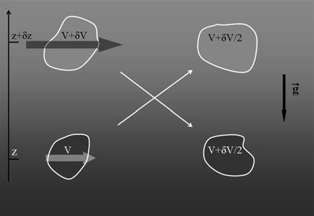
image credit: Maeder (2009), originally Talon (1997)
The Quest for a Good Initial Model
- should become shear unstable in stellar evolution code
- should not show other instabilities at the same time
- ideally similar time scale in stellar evolution and hydro code
a lot of work by R. Hirschi
- $20\,M_\odot$ ZAMS star, 40% crit. rotation
- core O burning phase
- Ne burning shell
- convectively stable
- Ri unstable
Simulation with GENEC

Simulations with SLH
- 2D equatorial plane
- more than 6 hours of physical time
- special mapping of GENEC data to keep convective stability
Evolution of Angular Momentum

Evolution of Mean Atomic Mass

Evolution of Richardson Number

First 3D work
by Leonhard Horst
- not straightforward to map model to 3D
- strict shellular rotation cannot always be upheld, while keeping a stable model
- some modifications to $\Omega$ profile to get a stable model in the equatorial plane
$\bar{A}$
Convective Overshooting in Pop III stars
collaborators:
Alexander Heger (Monash), Friedrich Röpke (HITS)
Setting
- zero metallicity initial model
- core He burning produced already significant amount of $^{12}\text{C}$
- H burning shell with $X(^{12}\text{C})=10^{-9}$
- convective core grows, reaches H burning shell
$250\,\msol$ star ($Z=0$) during core He burning

3D box (2013)
$128^3$ grid for about 4 days
Mach number
14N
energy release
3D wedge (2014)
$512^3$ grid
Next Steps
- start simulation right before overshooting reaches H shell
- include core using cubed sphere
Conclusions
- In many aspects stars should be treated as 3D, dynamical objects.
- SE codes are still needed to cover evolutionary timescale.
- Low Mach numbers require special numerical methods.
- Fully implicit, 3D hydro is possible and scales well to large supercomputers.
- We can now look at many poorly understood phenomena from stellar evolution in greater detail using hydro simulations.