Simulations of the LOcal Web (SLOW)
Latest constraints using new grouping and new bias correction
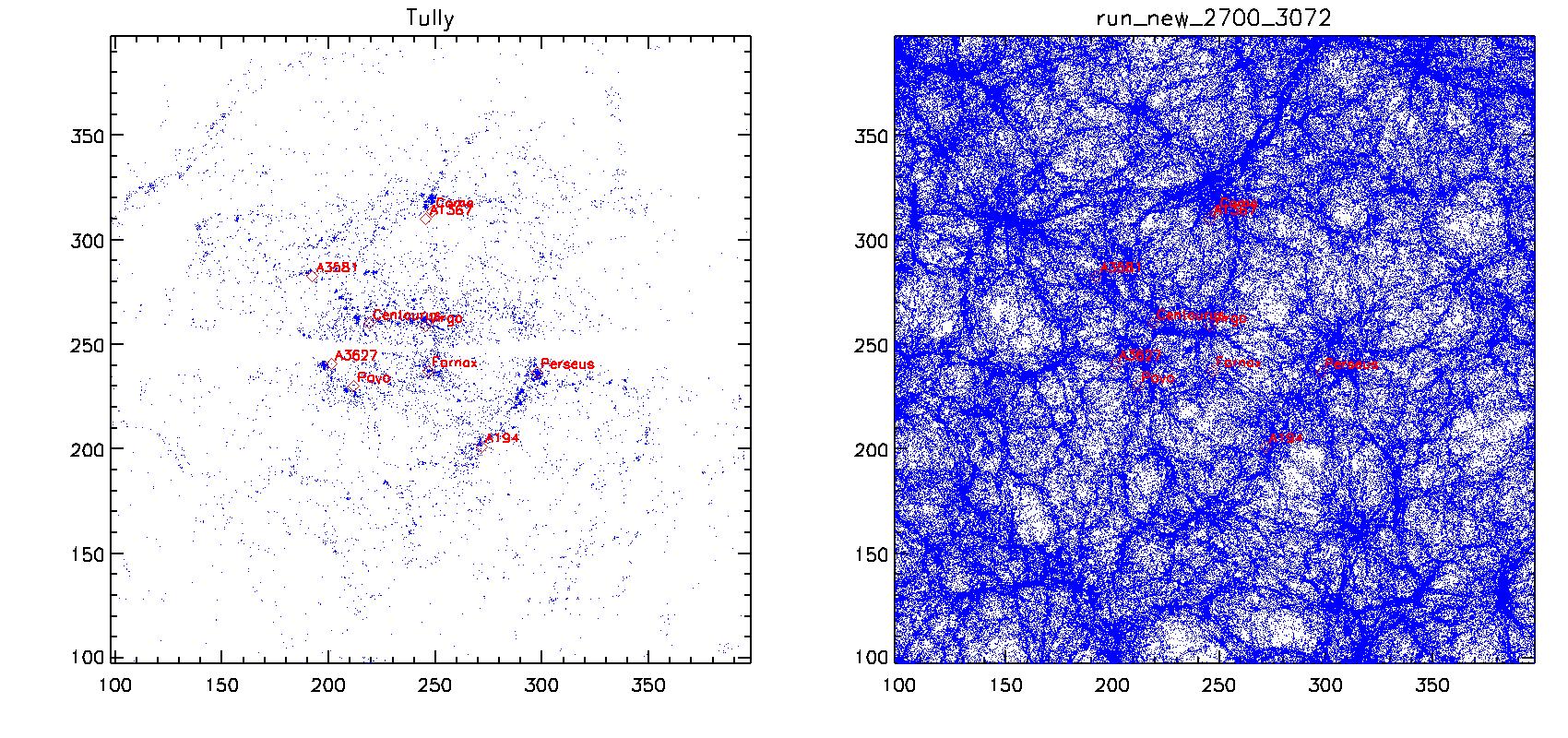
Thin slice through the local universe. Left side: Galaxies from the Tully catalog and prominent Abel clusters from NED.
Right side: Galaxies in the simulation and prominent Abel clusters from NED.
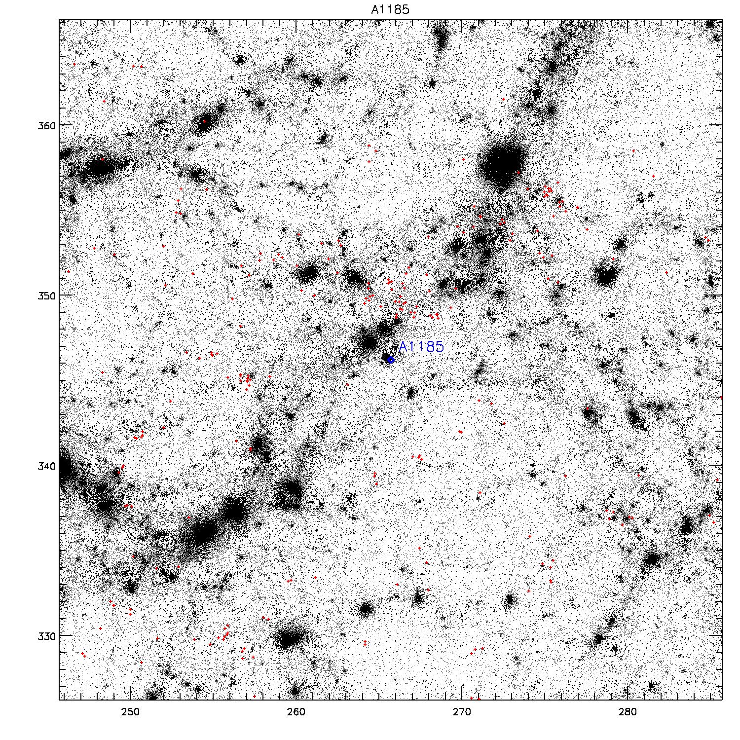
Comparison of the structures in the simulation arround local Abel clusters (from NED) and positions of galaxies
from the Tully catalog.
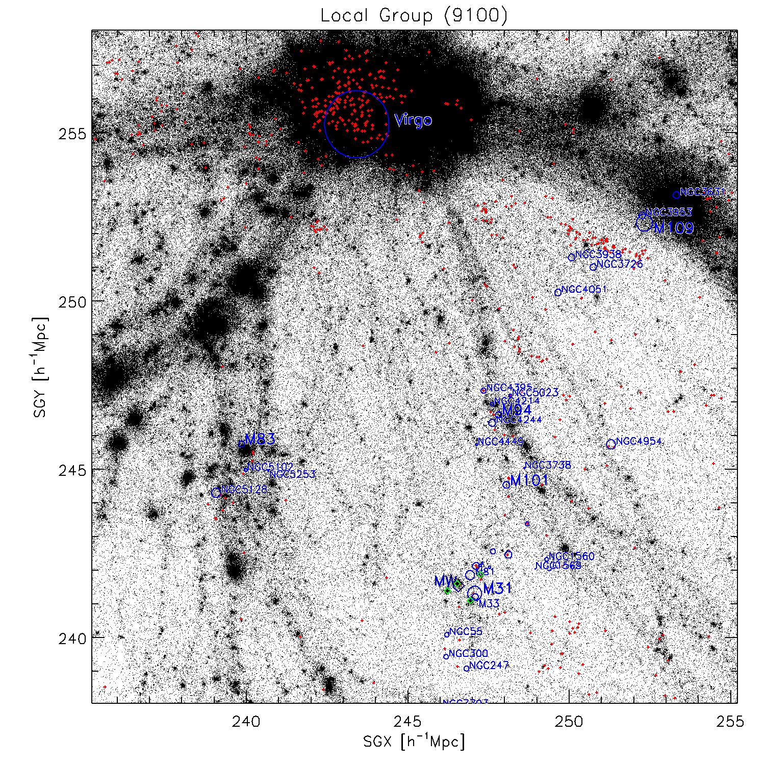
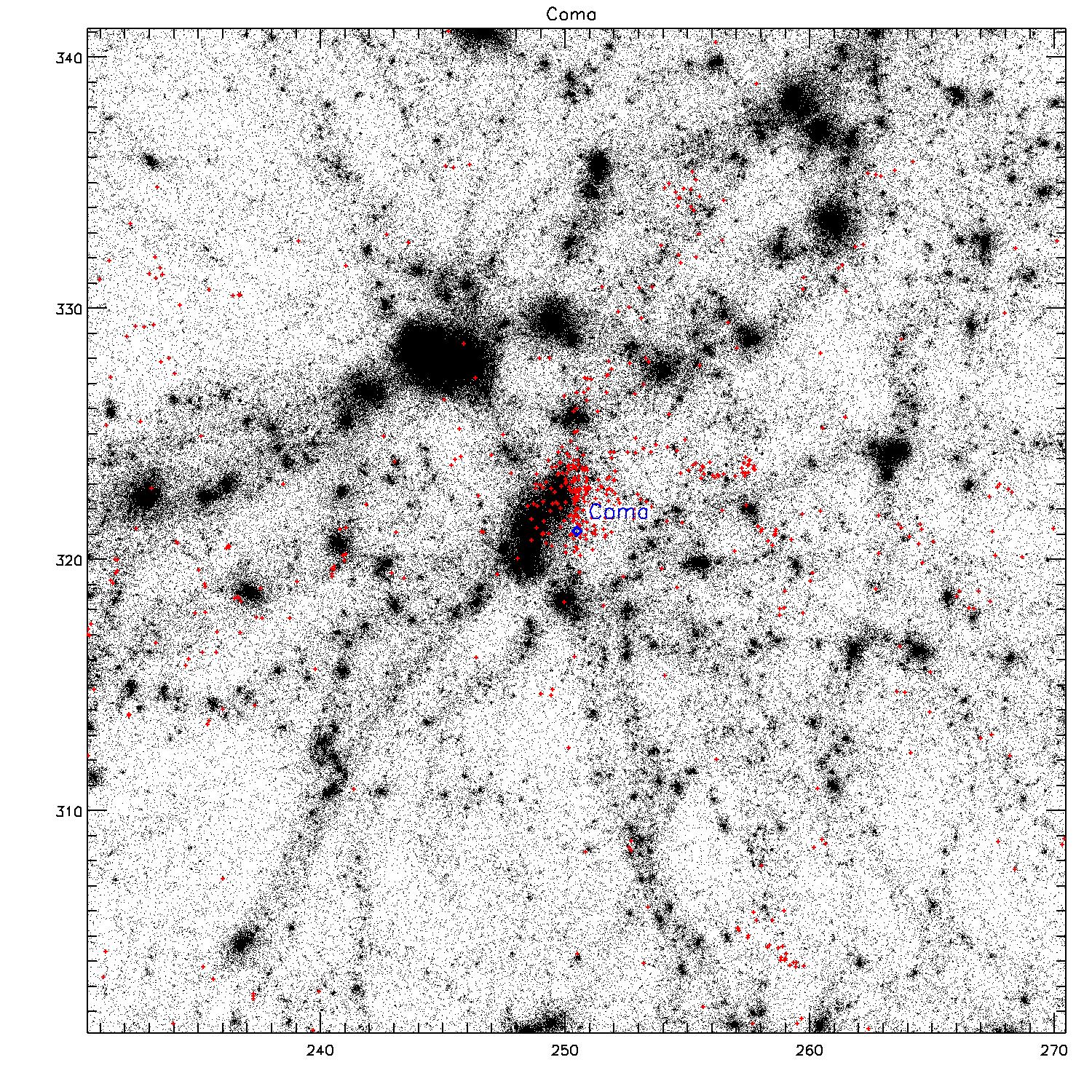
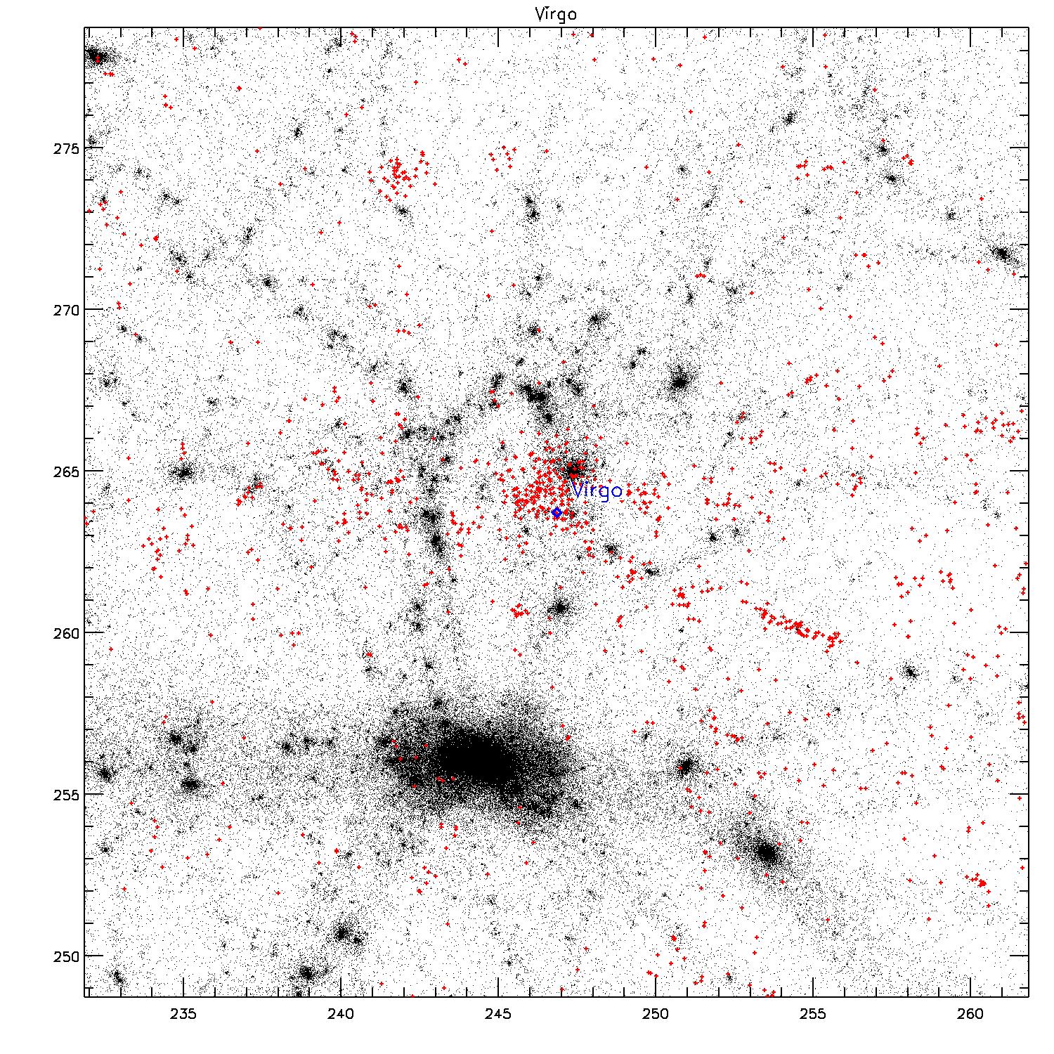
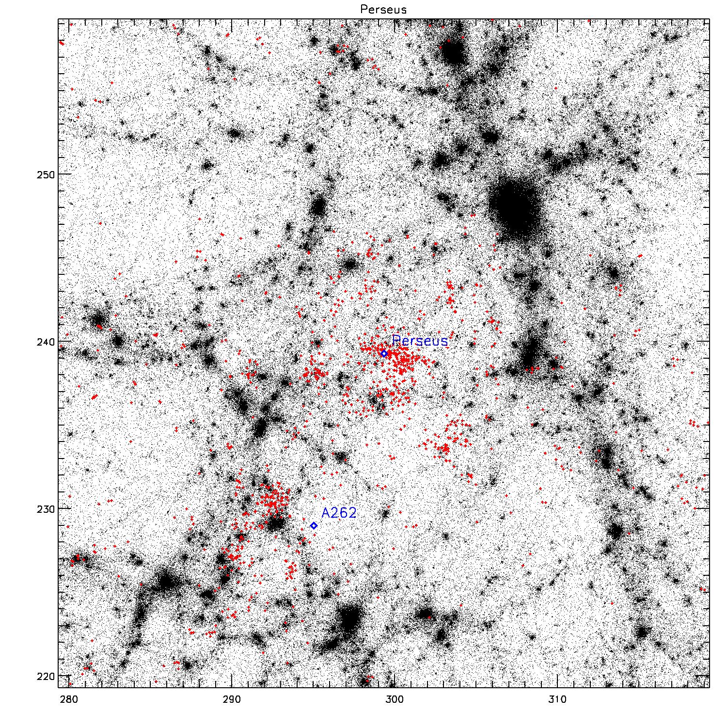
Thin slice through the local group. Black: Simulation; Red: Galaxies from the Tully catalog; Blue: Prominent Galaxies from NED.
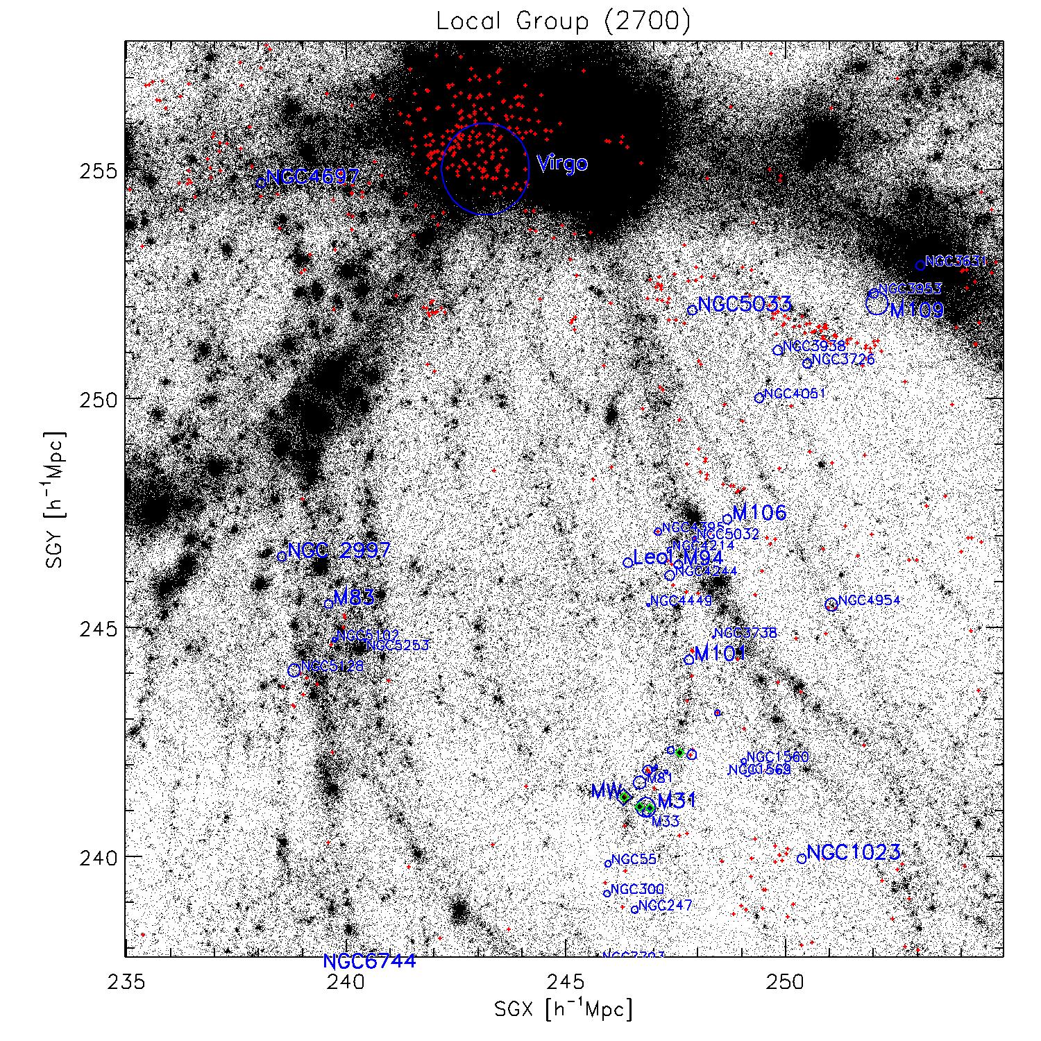

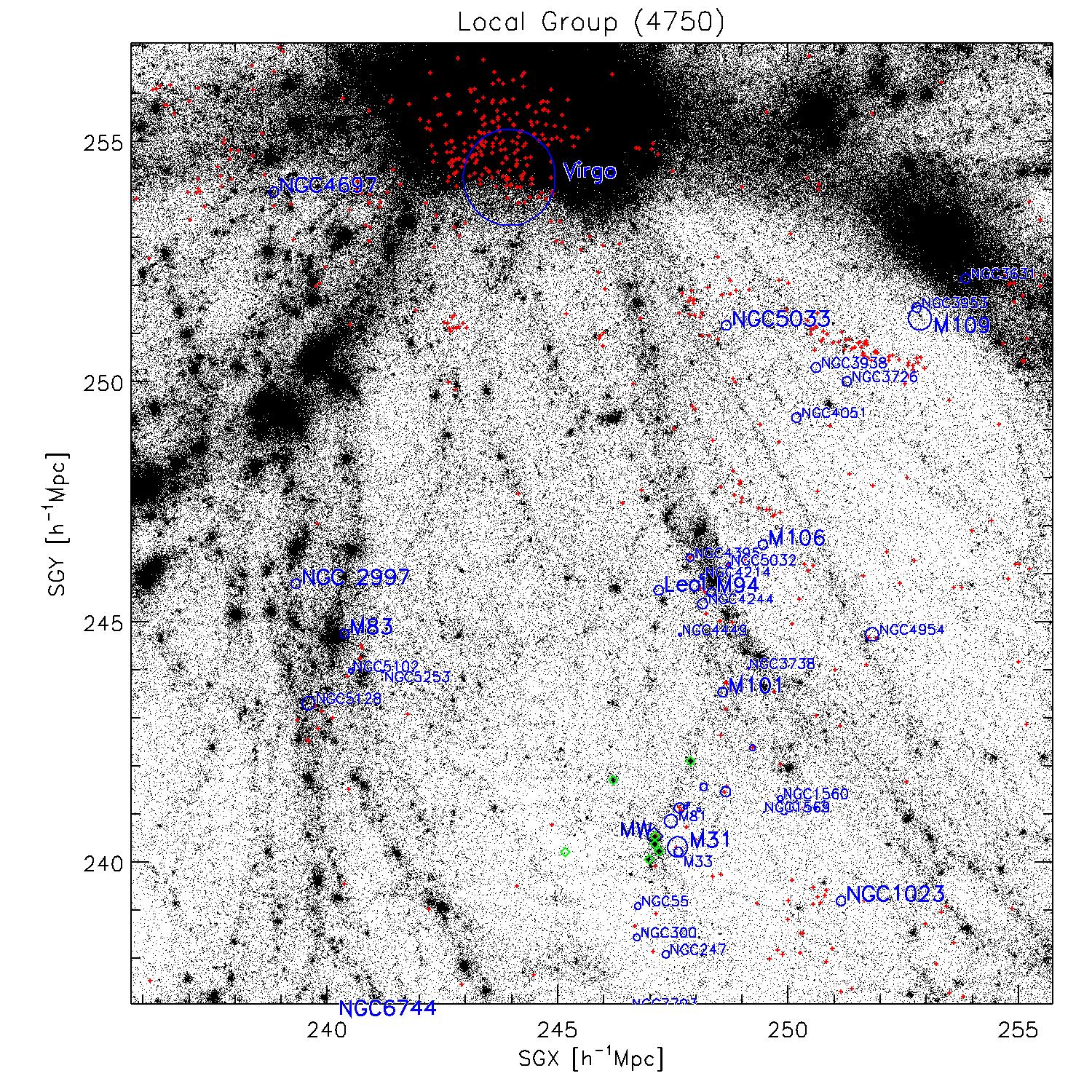


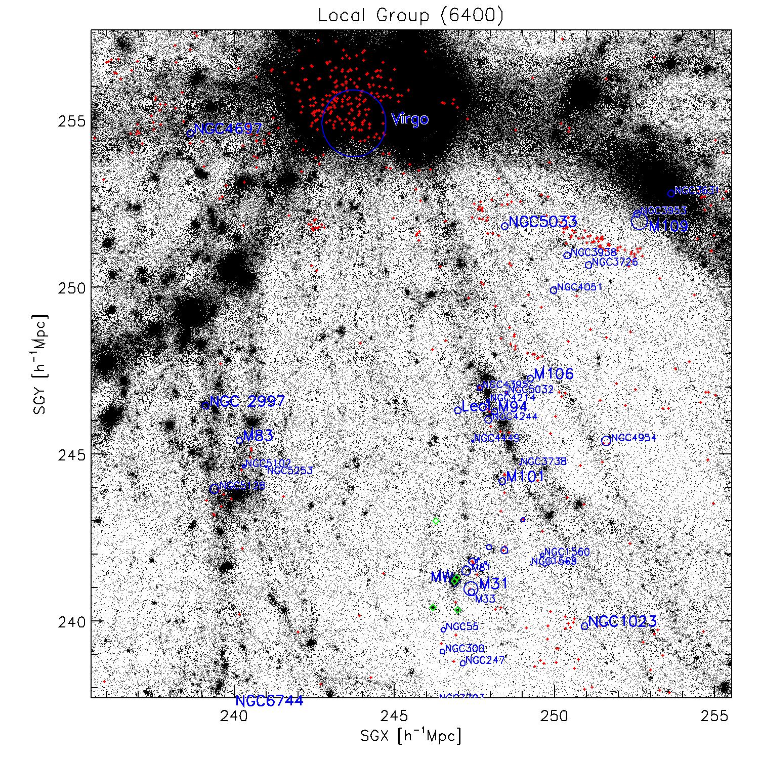

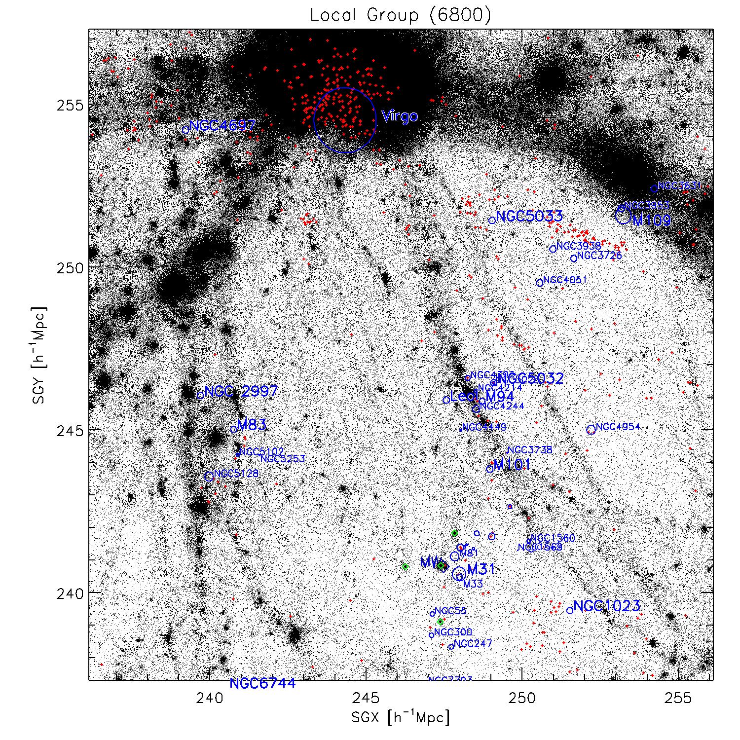
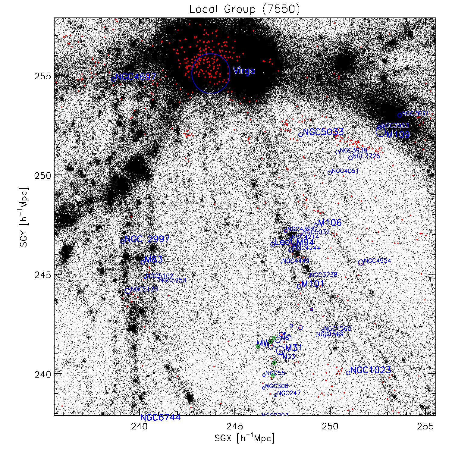
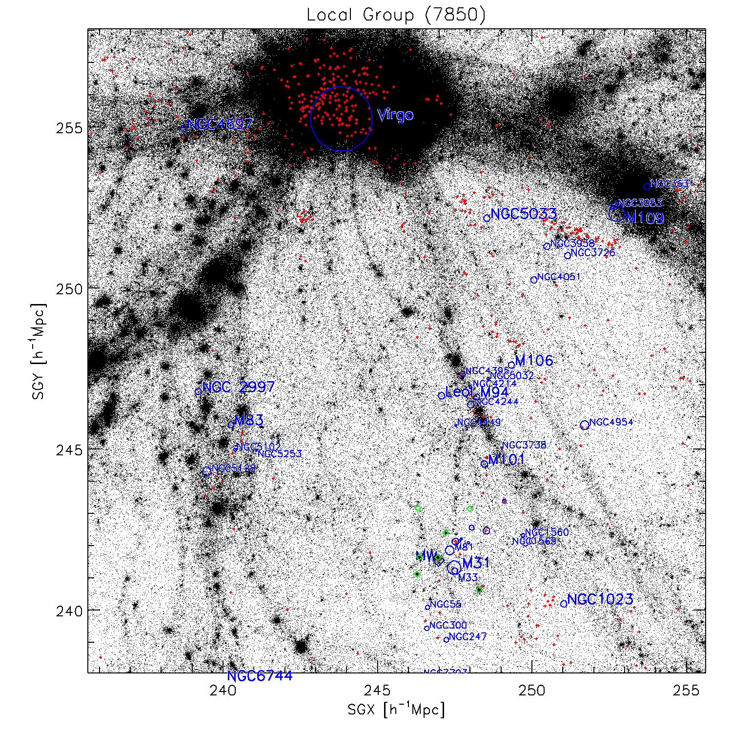
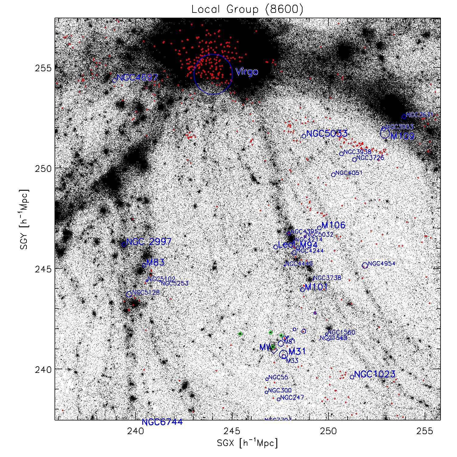
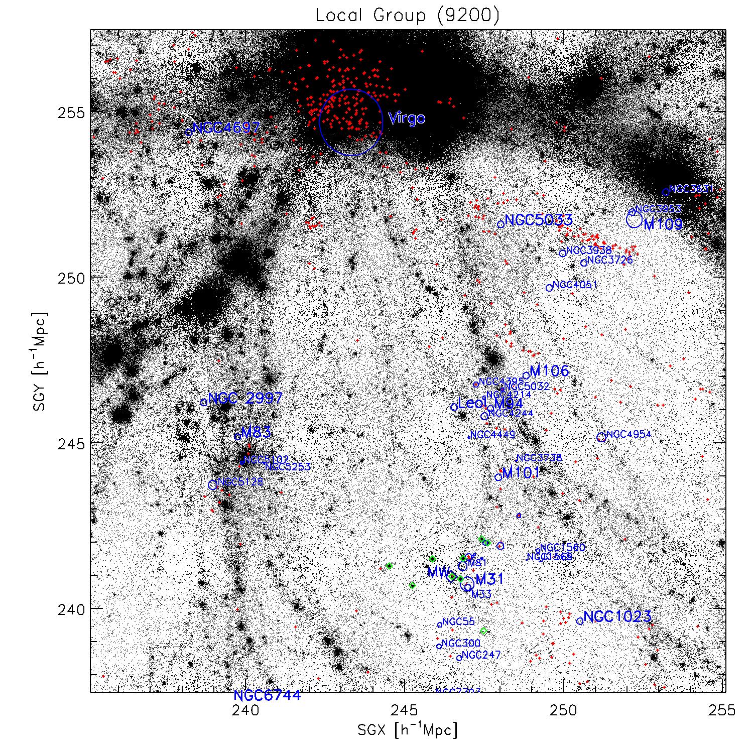
Same as before, but for different random realizations.
First attempts using original grouping and bias correction
Varying large scale seed for reconstruction
Mean over 200 simulations (left) and animation over the 200 realisations on the right. Upper row is the local environment, lower row the large scale matter distribution. Red symbols mark groups and clusters from the Tully 2016 catalogue. Click on image to enlarge.
Varying small scale seed for reconstruction
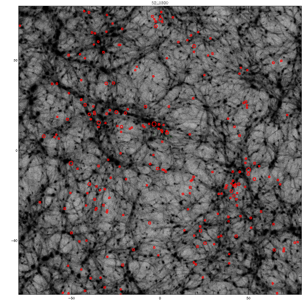
Mean over 50 simulations with varying small scale random field (left) and animation over the 50 realisations on the right. Upper row is the local environment, lower row the large scale matter distribution. Red symbols mark groups and clusters from the Tully 2016 catalogue. Click on image to enlarge.
Full sky Maps of 52_2600_3072
Full sky maps of the galaxy distribution from the 52_2600 simulation (left), from the 2MRS galaxy catalouge (middle) and from the Matthis et al. 2002 simulation (right).
For the simulations, v_max is used to estimate Mk=-2.34-8.16*alog10(2*v_max) and then M=m-25-5*alog10(d[Mpc]) is used to do a magnitude cut at m_k=11.75 to be consistent with teh observations.
Rows (from top to bottom): 5-20 Mpc, 20-50 Mpc, 50-120 Mpc and 120=250 Mpc.
Comparison of galaxies
Shown is a thin slice across the super-galactic plane using the galaxies in the 2MKS (upper left),
the galaxies from the 52_2600 (lower left), the 66 (selection of Jenny, lower right) and the
Mathis et al. 2002 simulation (upper right). For the simulations a magnitude cut
as in the observations, based on vmax and distance, is always applied. The blue contours are
smoothed density contours from the 2MKS catalogue.
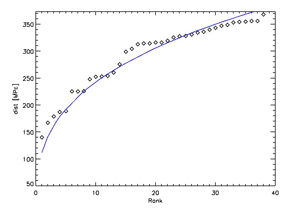
Comparison of mass function
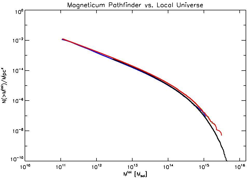
Shown is the cumulative halo mass function from magneticum (blue and black) and the local universe
simulation (red) which resonable well agree. The problem here is, that within the (500Mpc/h)^3
volume we find 67 clusters with Mvir>1e15Msol (as expected). However, in the local universe
Tully reported 5 clusters with M>1e15Msol in his catalouge. I checked the distances:
Norma, 61 Mpc, Perseus 70 Mpc, Coma 80 Mpc, Ophiuchus 116 and A2199 118 Mpc. Given the
mass function we would expect 1 such cluster within 112 Mpc and to have 5 such clusters, we
should need to go to a sphere with radius of 192 Mpc. Now it gets spuky: The ranked distances
of cluster with such masses are: 140.204, 167.453, 178.911, 187.476, 189.061, 225.135, 225.139,
225.694, 248.093 ...
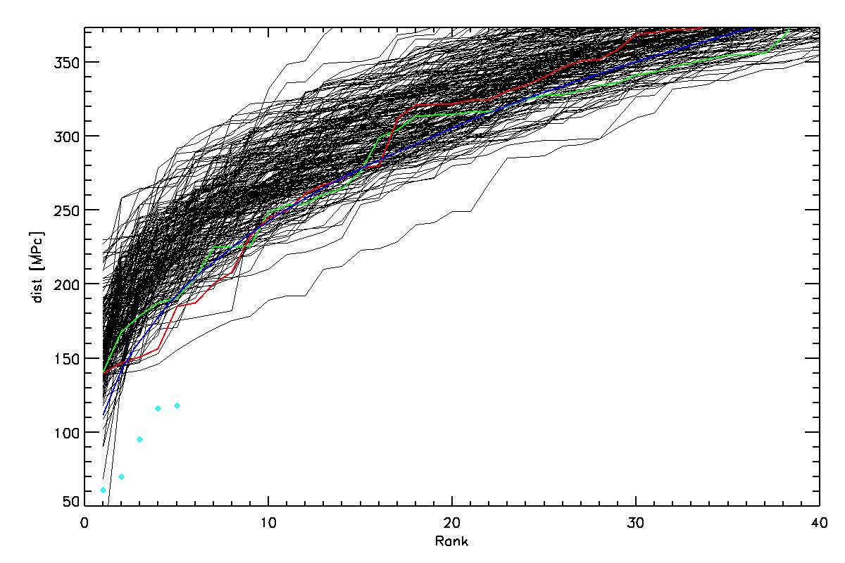
Same as before but for all 200 realizations. Green is 52, red is 66 and blue diamonds are the
5 massive clusters from the Tully catalouge.
Comparison of mass of known objects
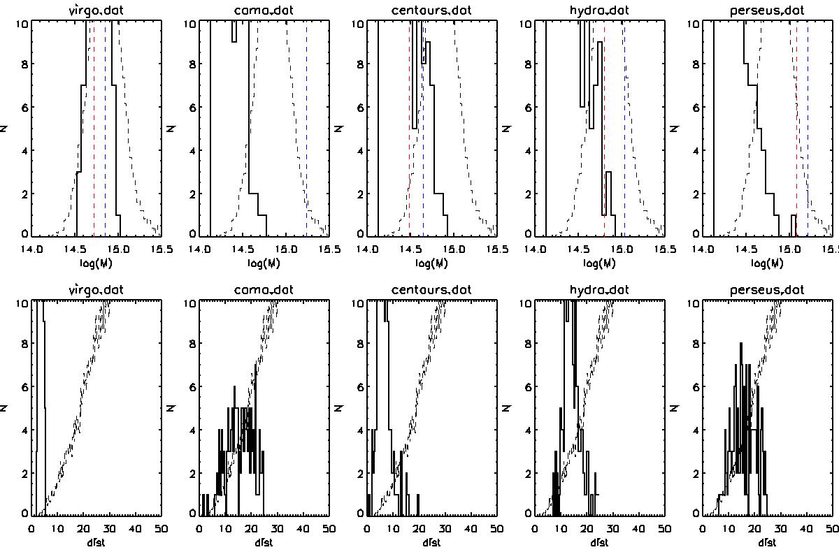
Shown are the distribution of the mass (upper row) and distance to the real position (lower row)
of well known clusters over the 200 realizations (black histograms). The dashed histograms (upper row)
are the distribution of masses of clusters above 1.5e14 Msun/h found closest to random points in
space and the dashed histograms in the lower row are their typical distance and can be used
to interpreted the chance of randomly finding a cluster of such mass. Position of virgo, centaurus
and hydra are very good constrained (in contrast to coma and perseus) but the used constrains
are forcing coma and perseus to be to less massive, which can be seen comparing to the blue and red
dashed lines, indicating the mass of the systems from Tully catalogue and x-ray measurements.
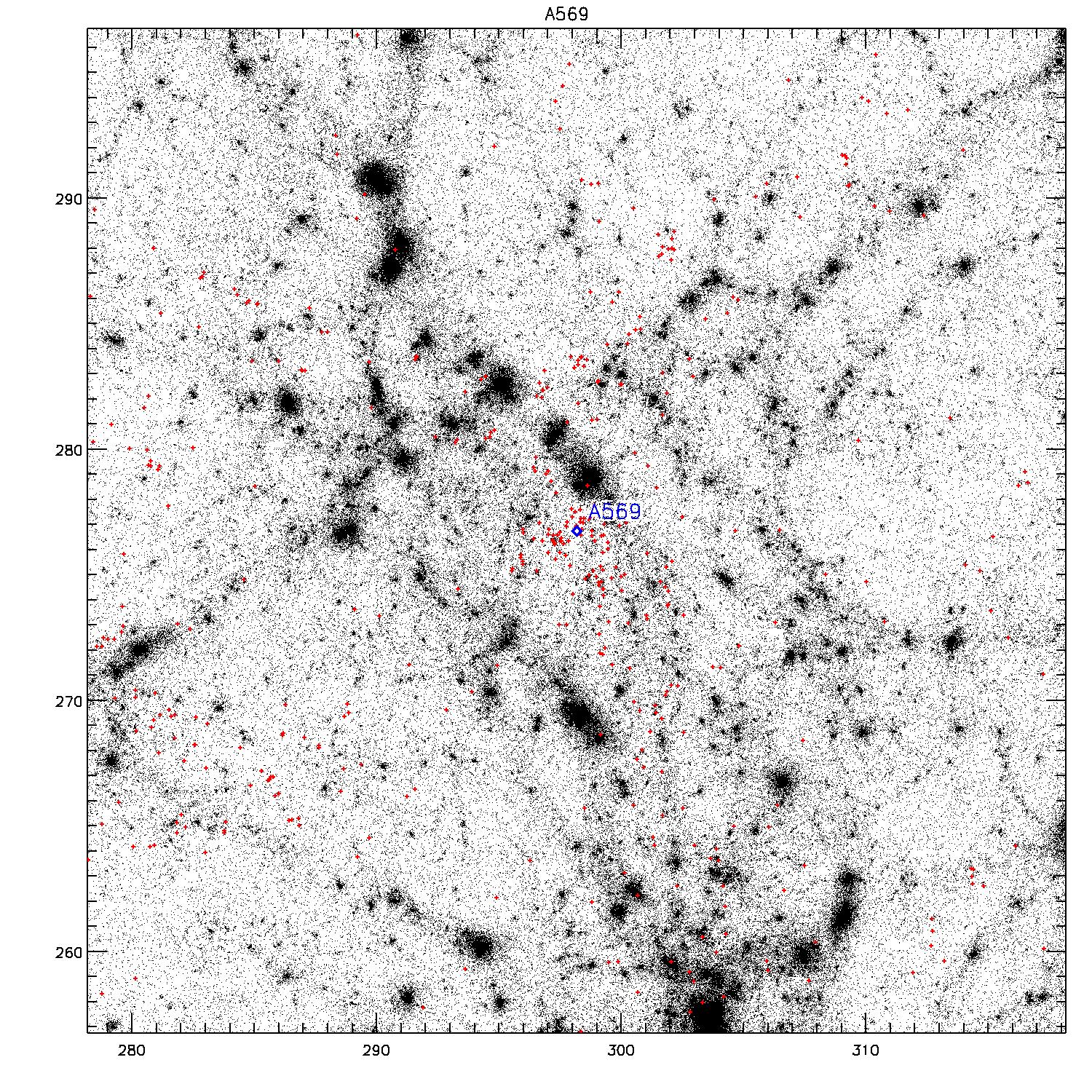
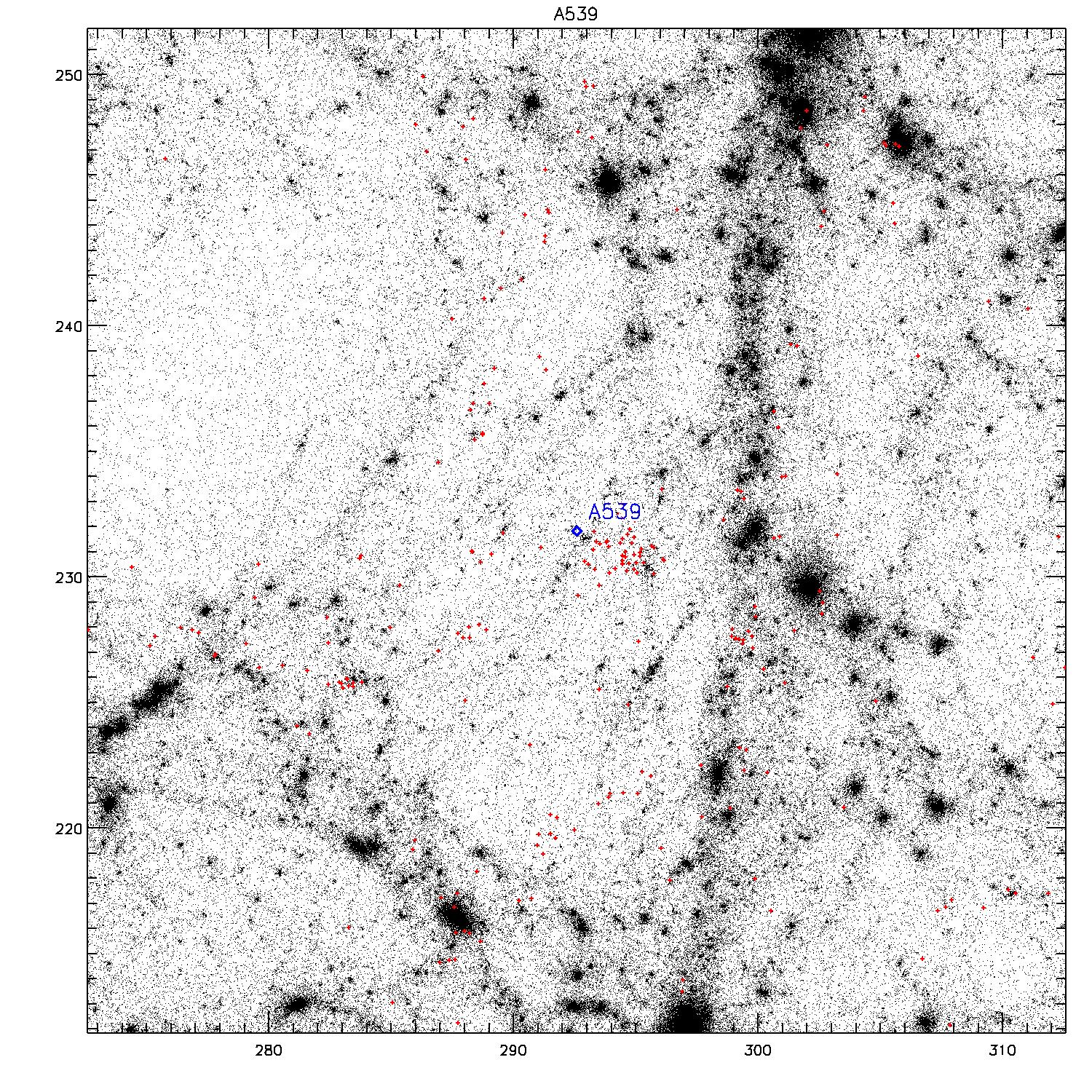
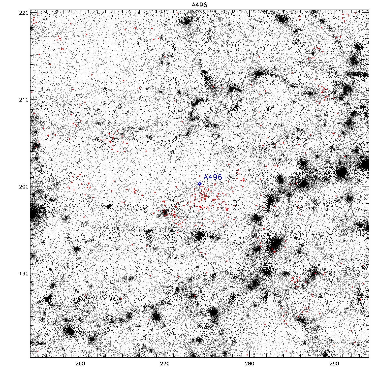
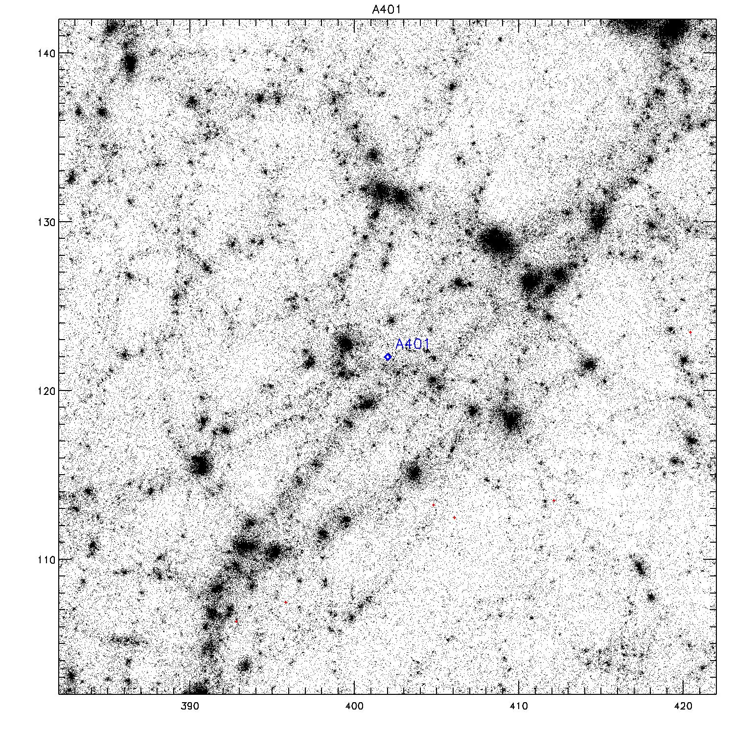
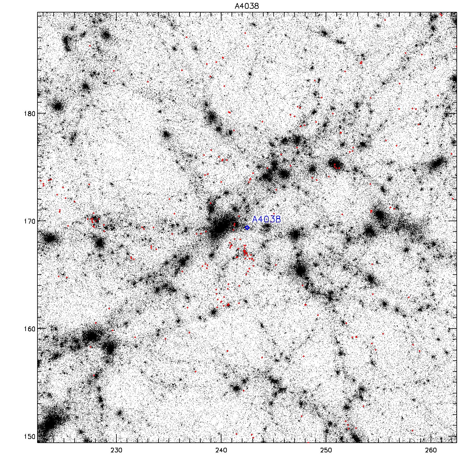
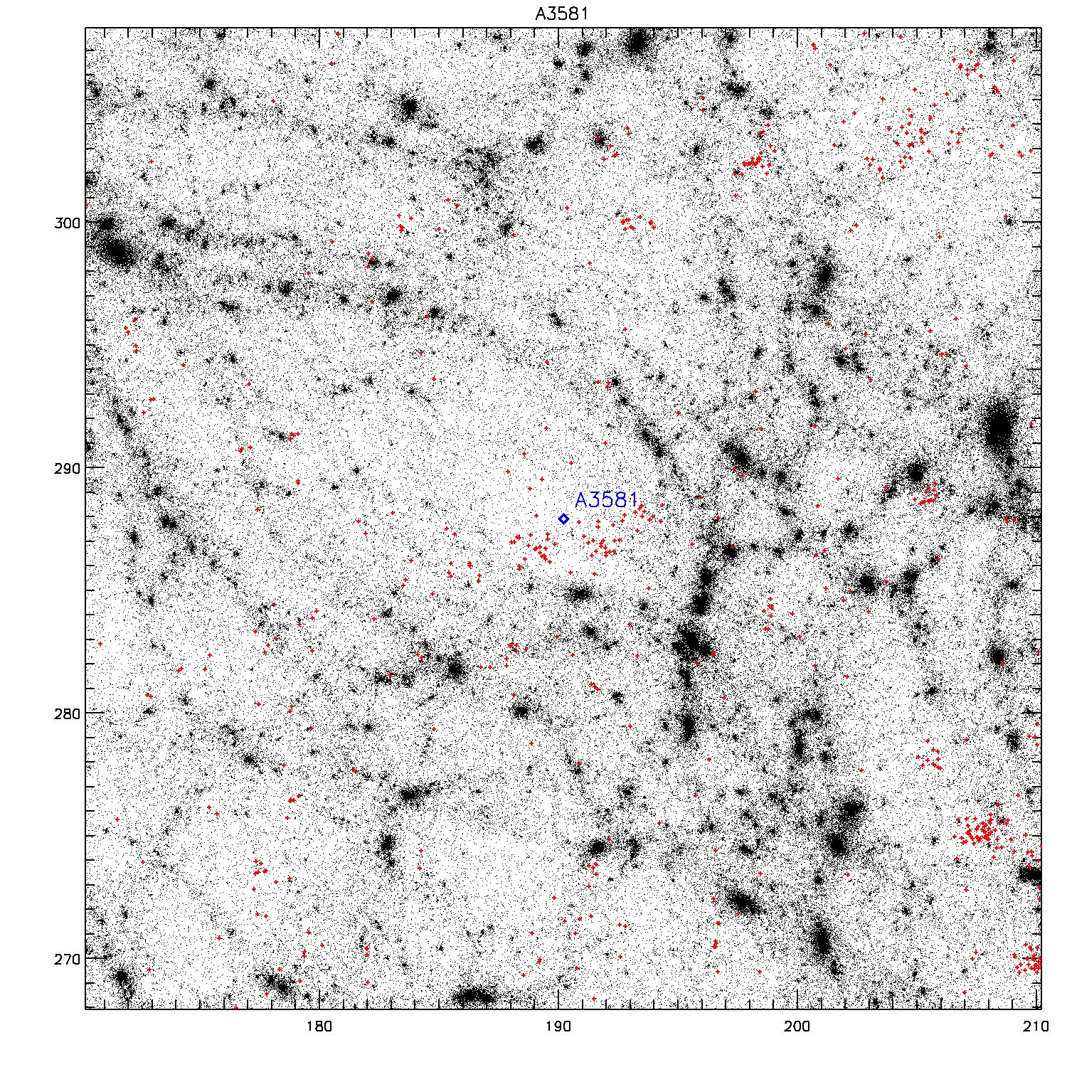
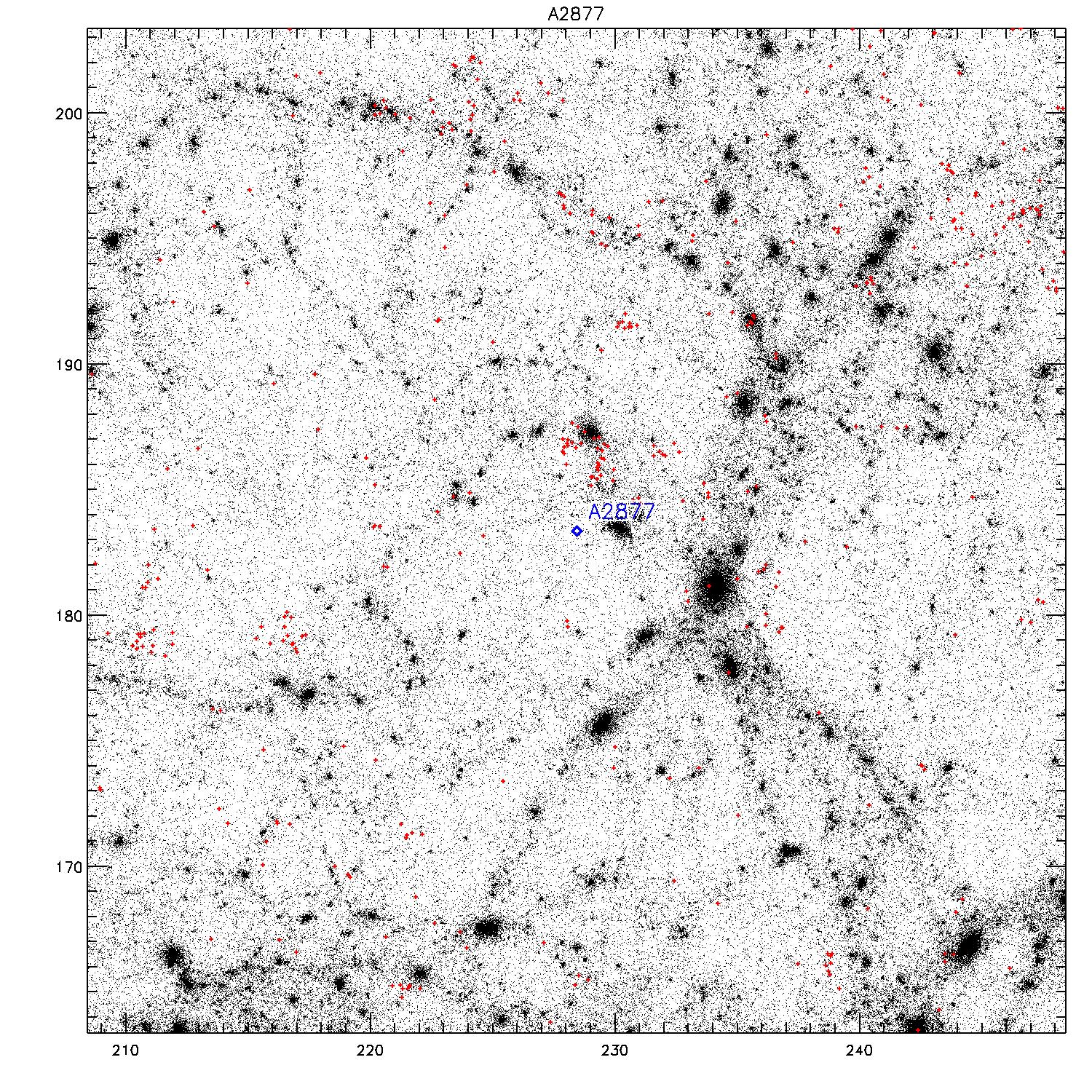
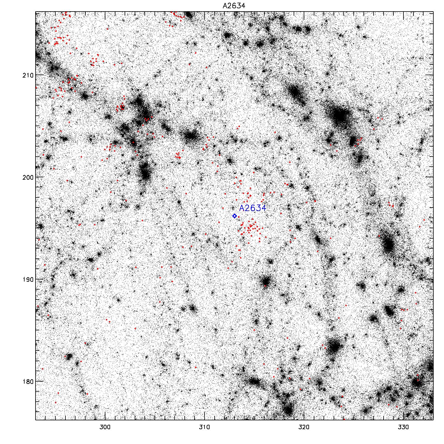
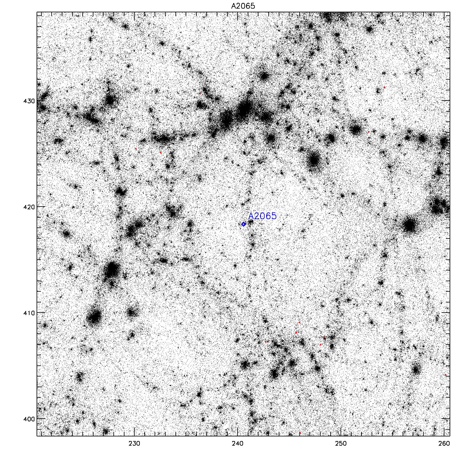
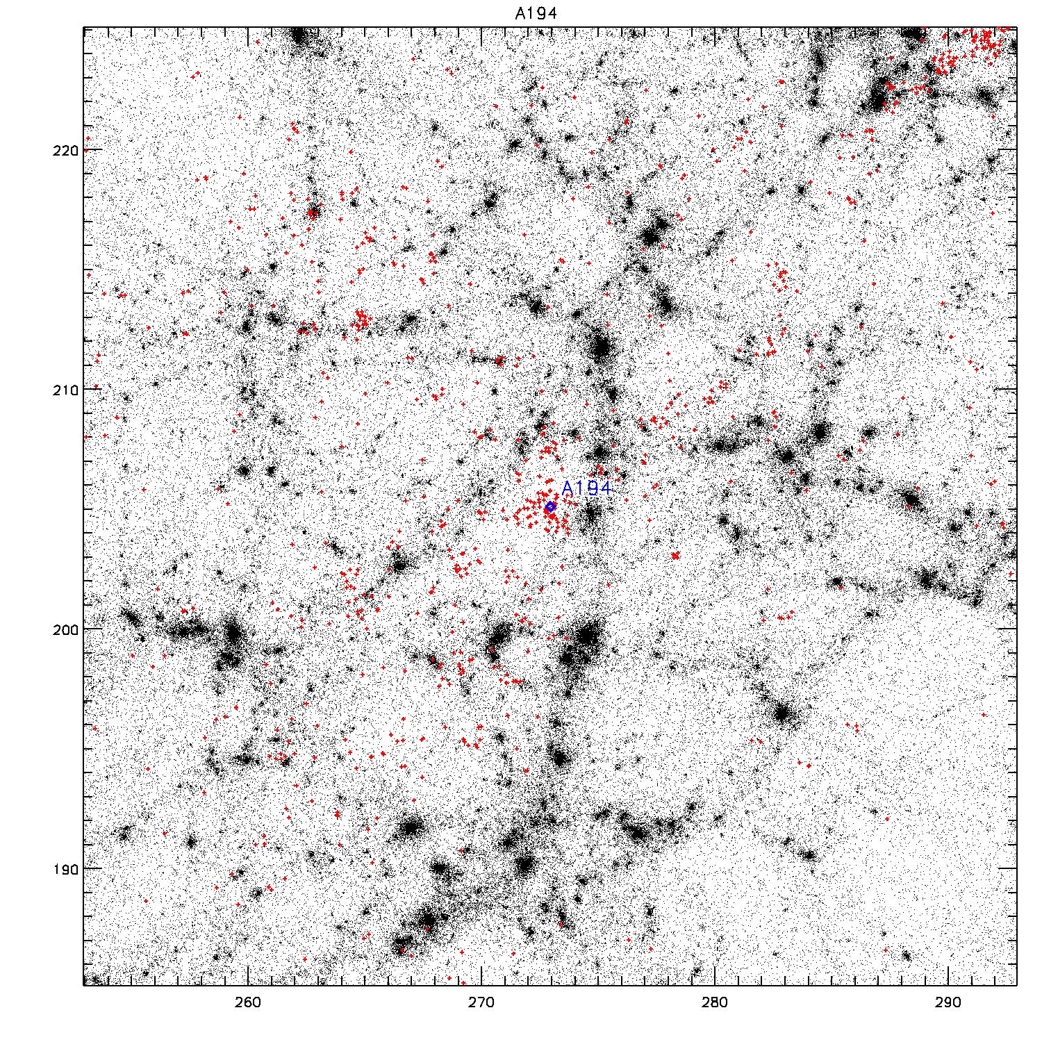
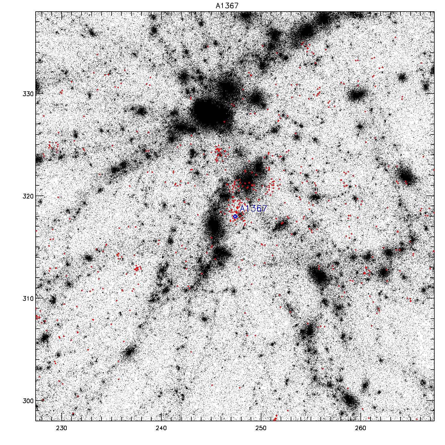
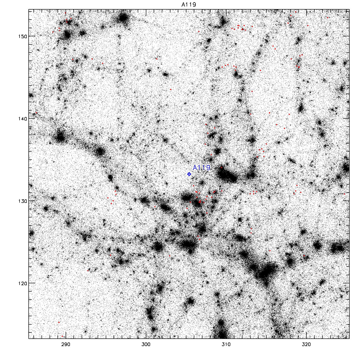
Individual comparions
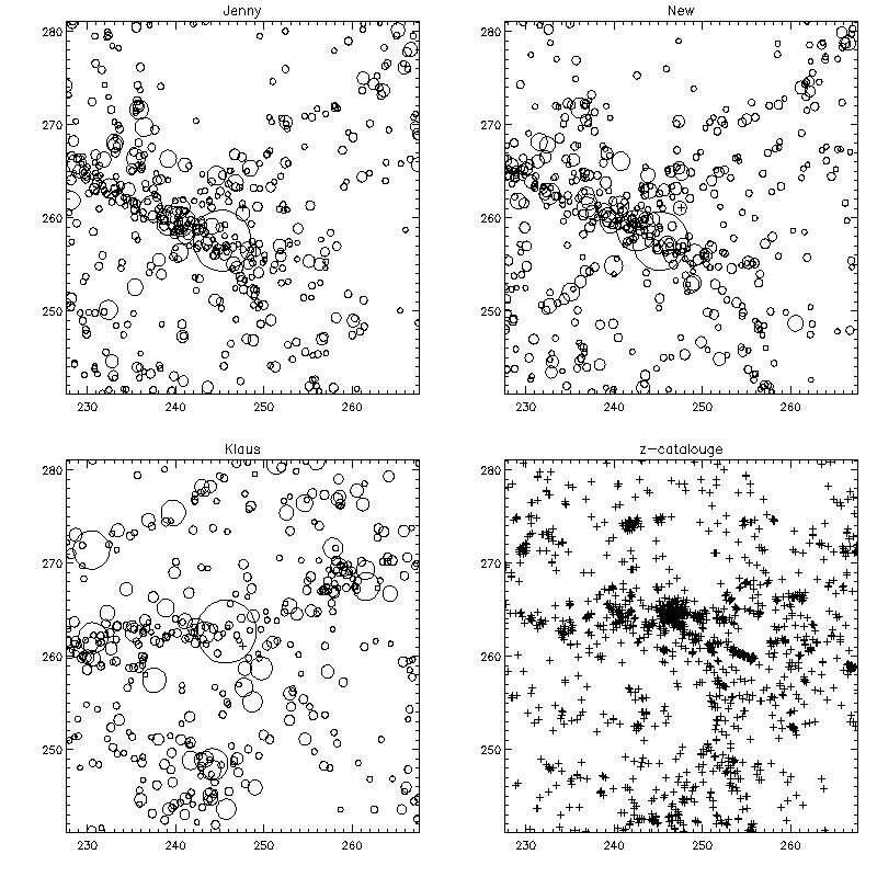
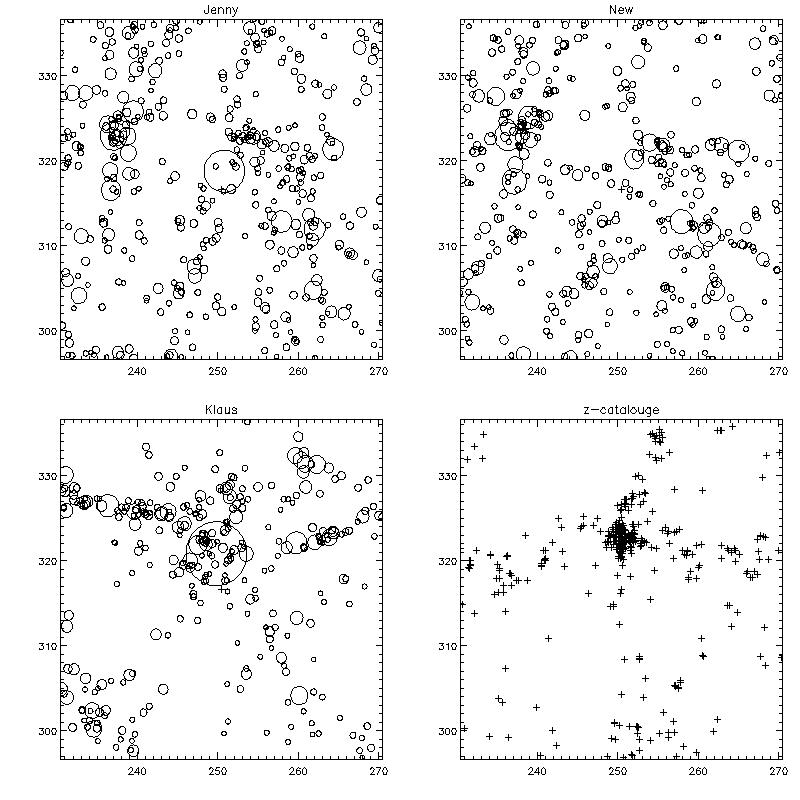
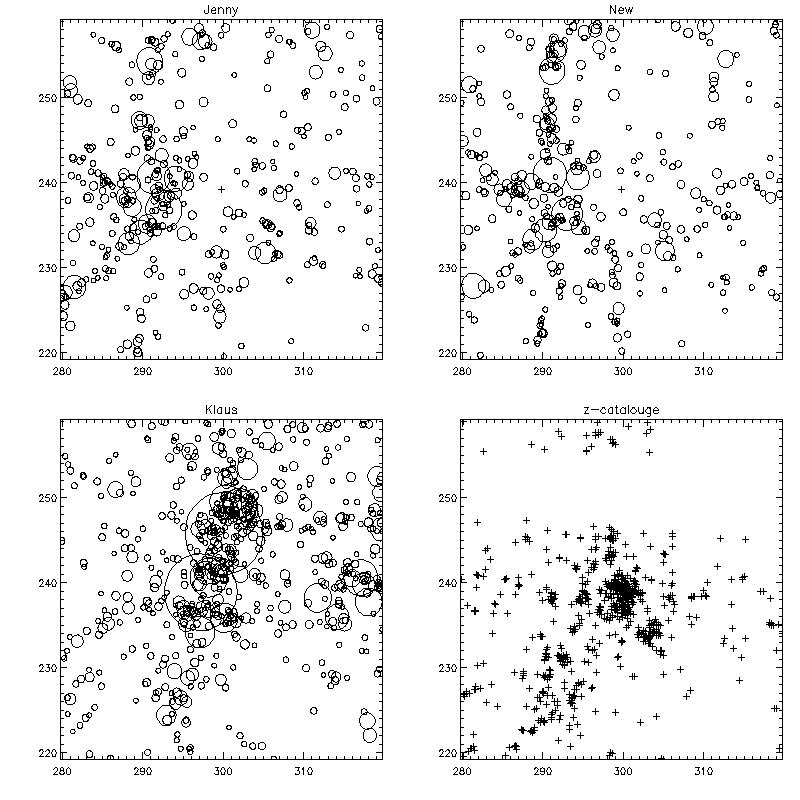
Position and size of haloes within the 66 (Jenny), the 52 (New), the Matthis 2002 (Klaus)
and galaxies in the 2MKS (z-catalogue) for virgo (upper plot), coma (middle plot) and
perseus (lower plot).
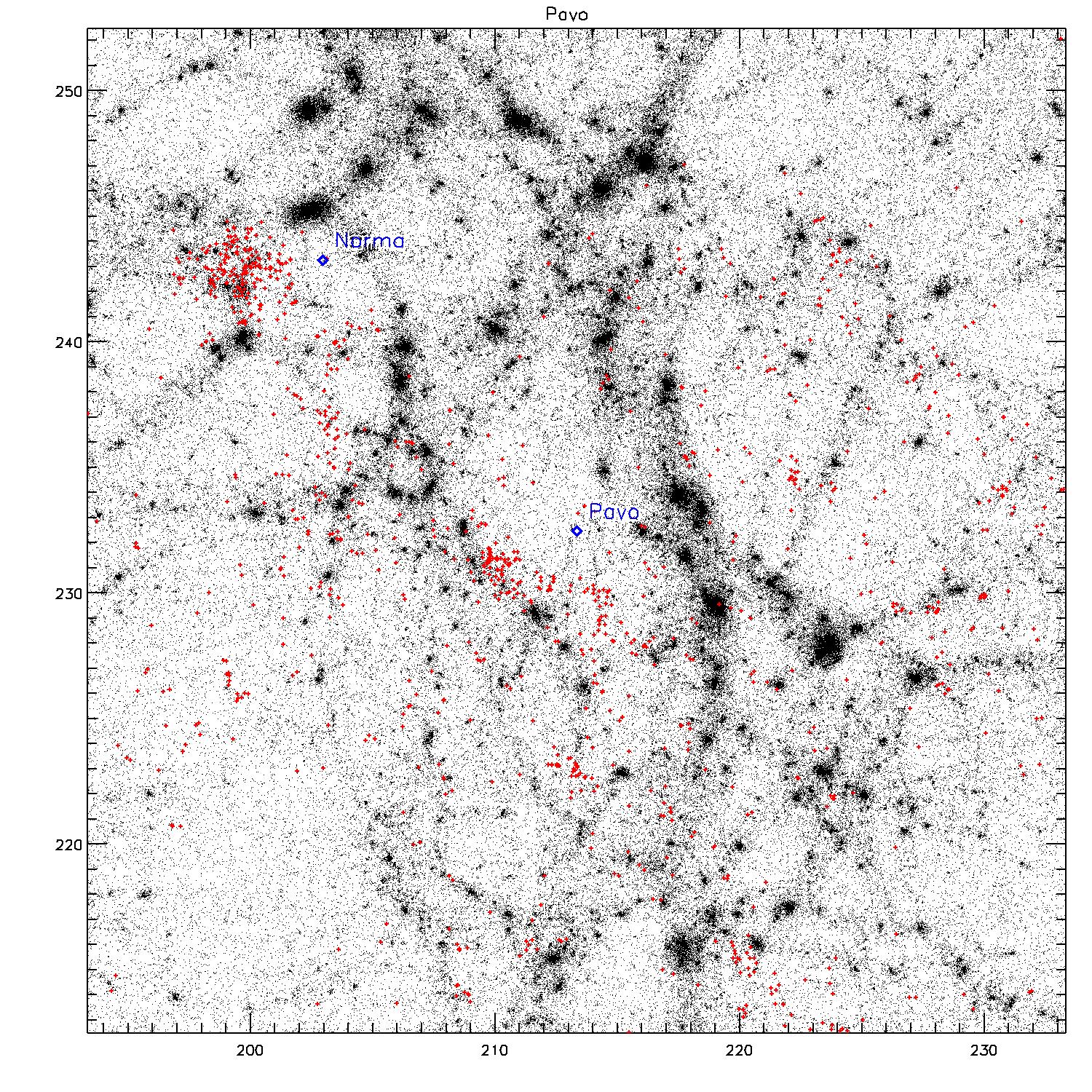
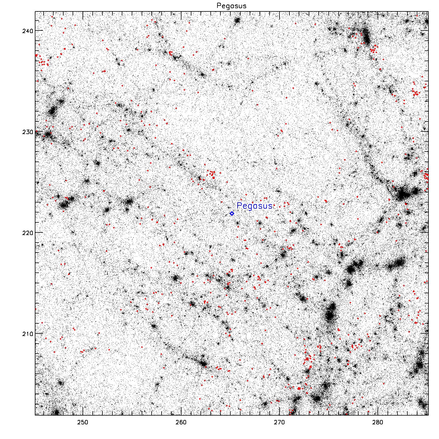
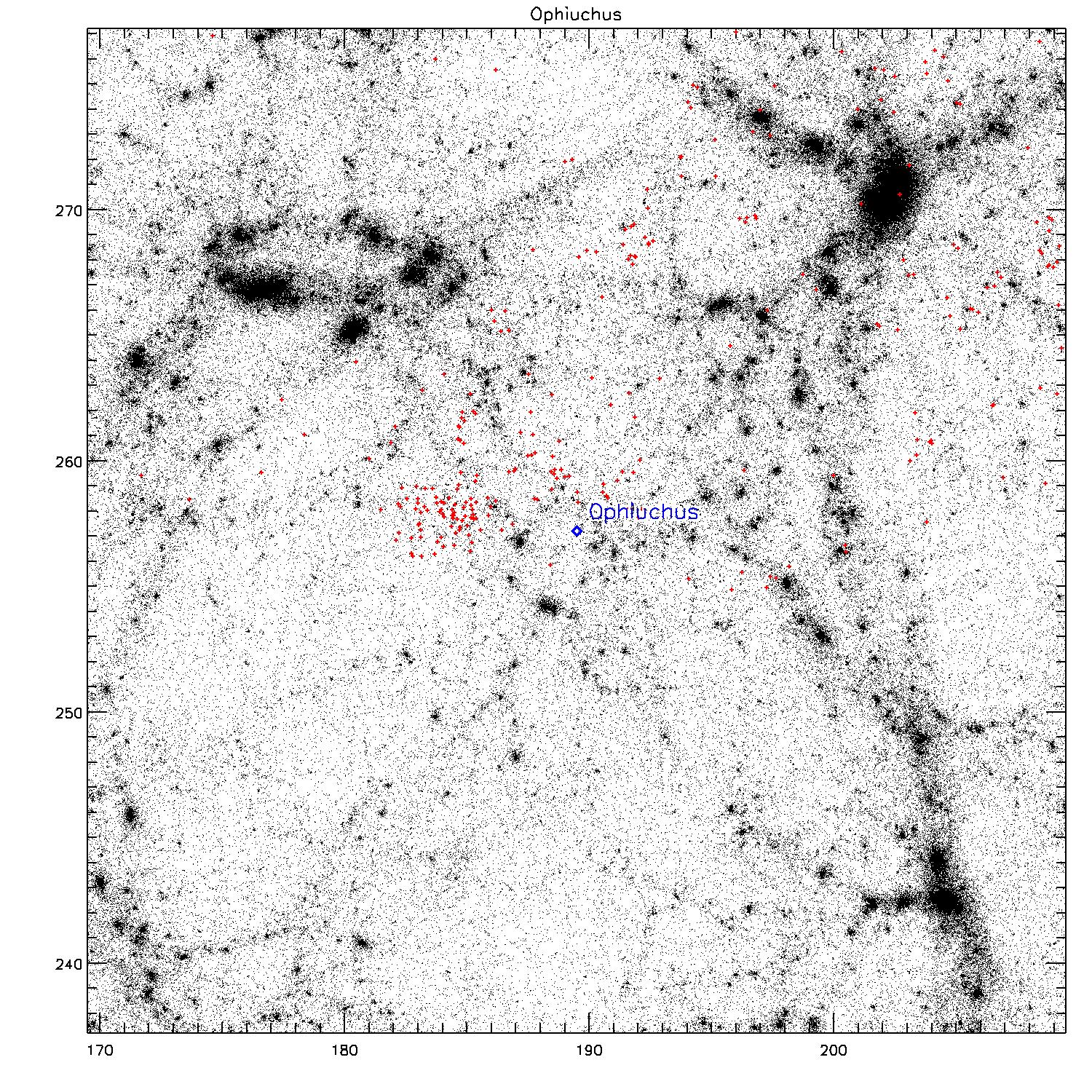
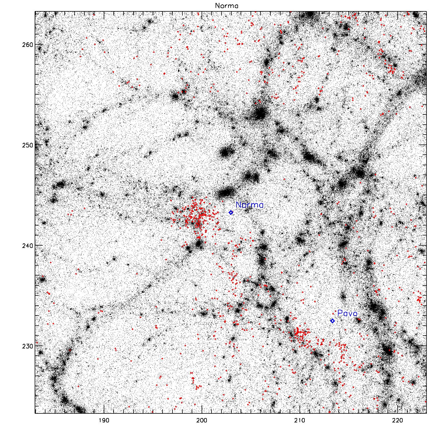
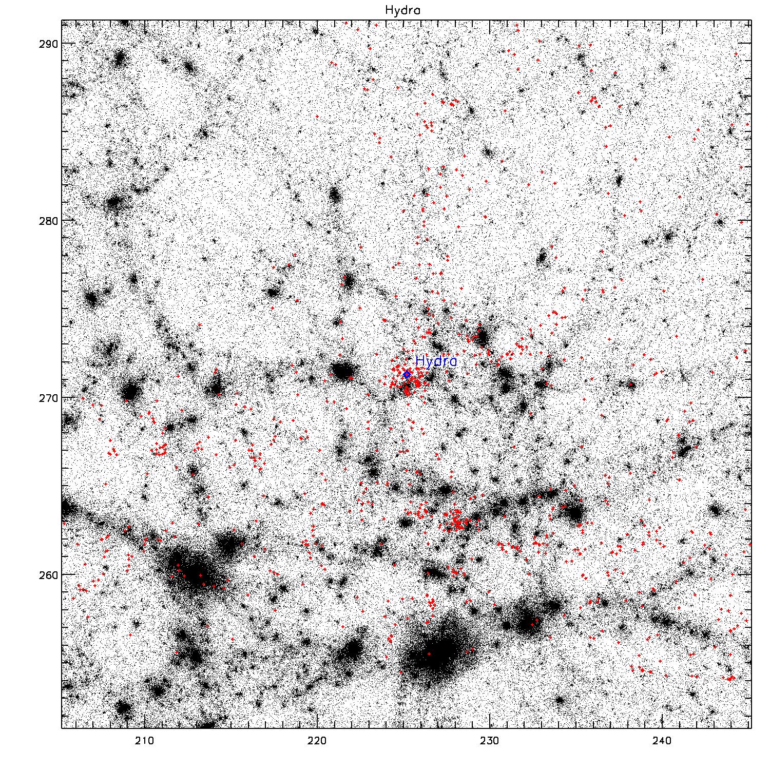
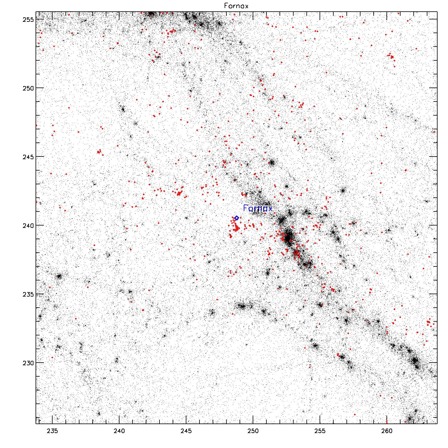
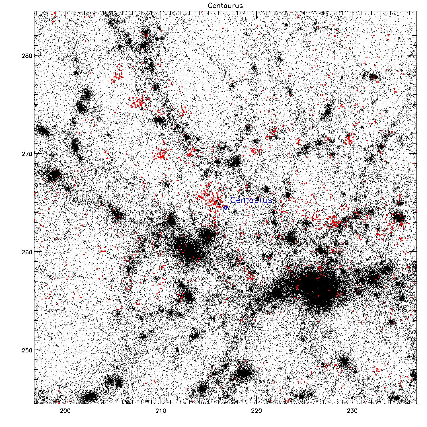
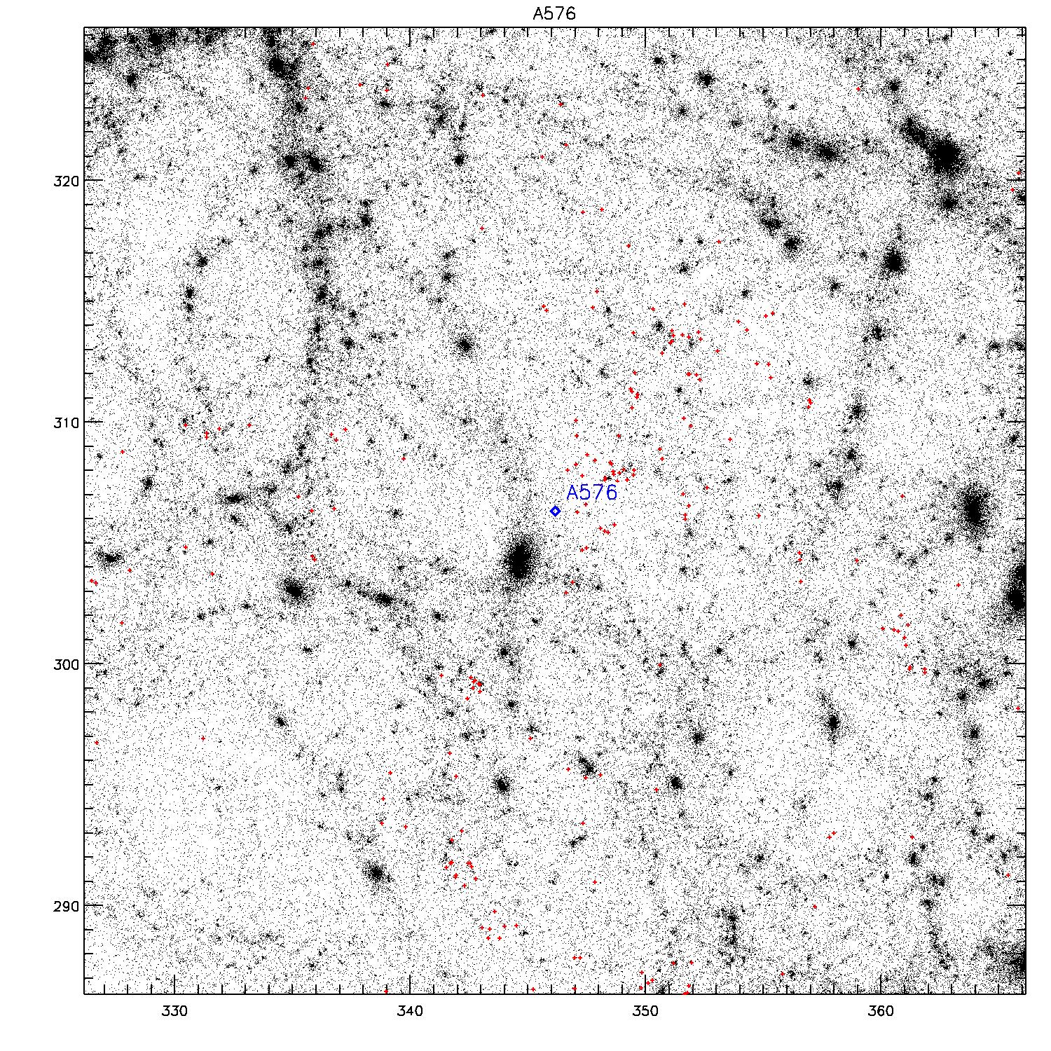
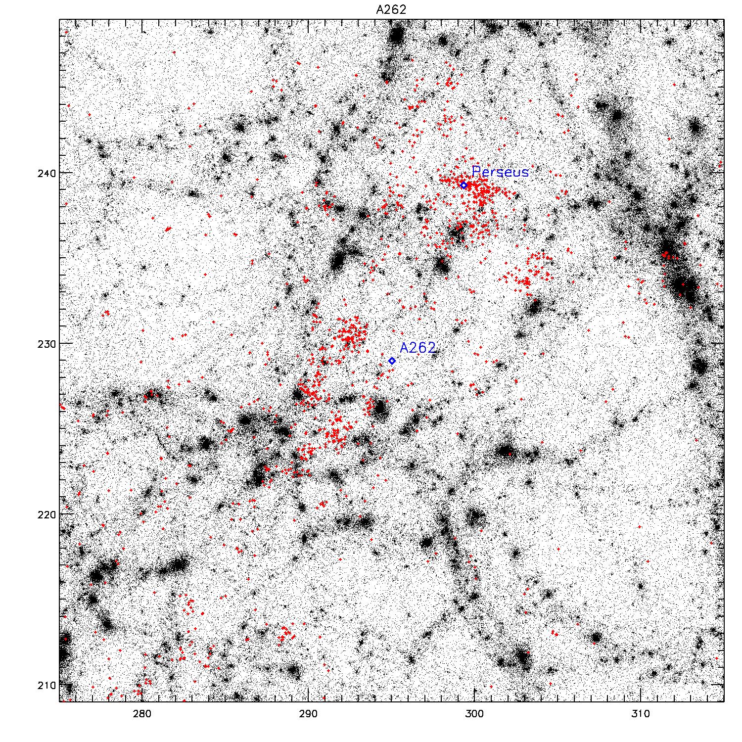
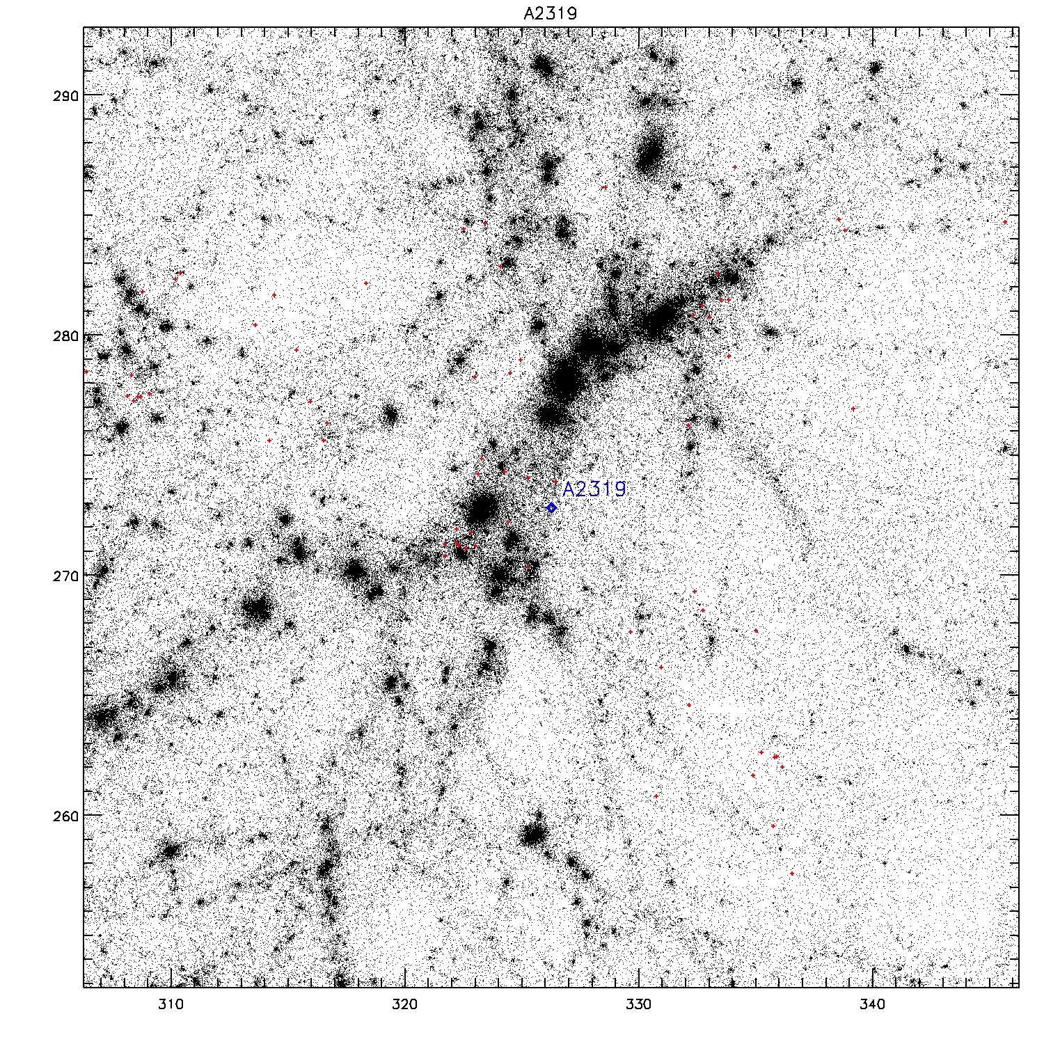
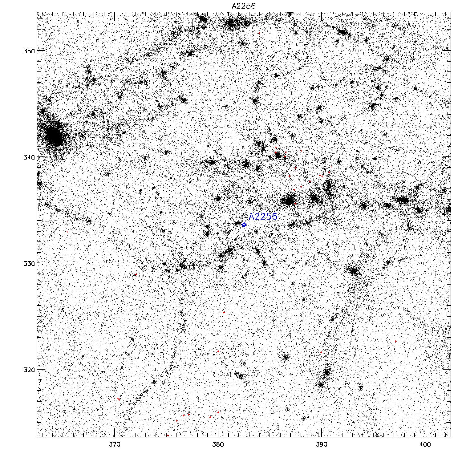
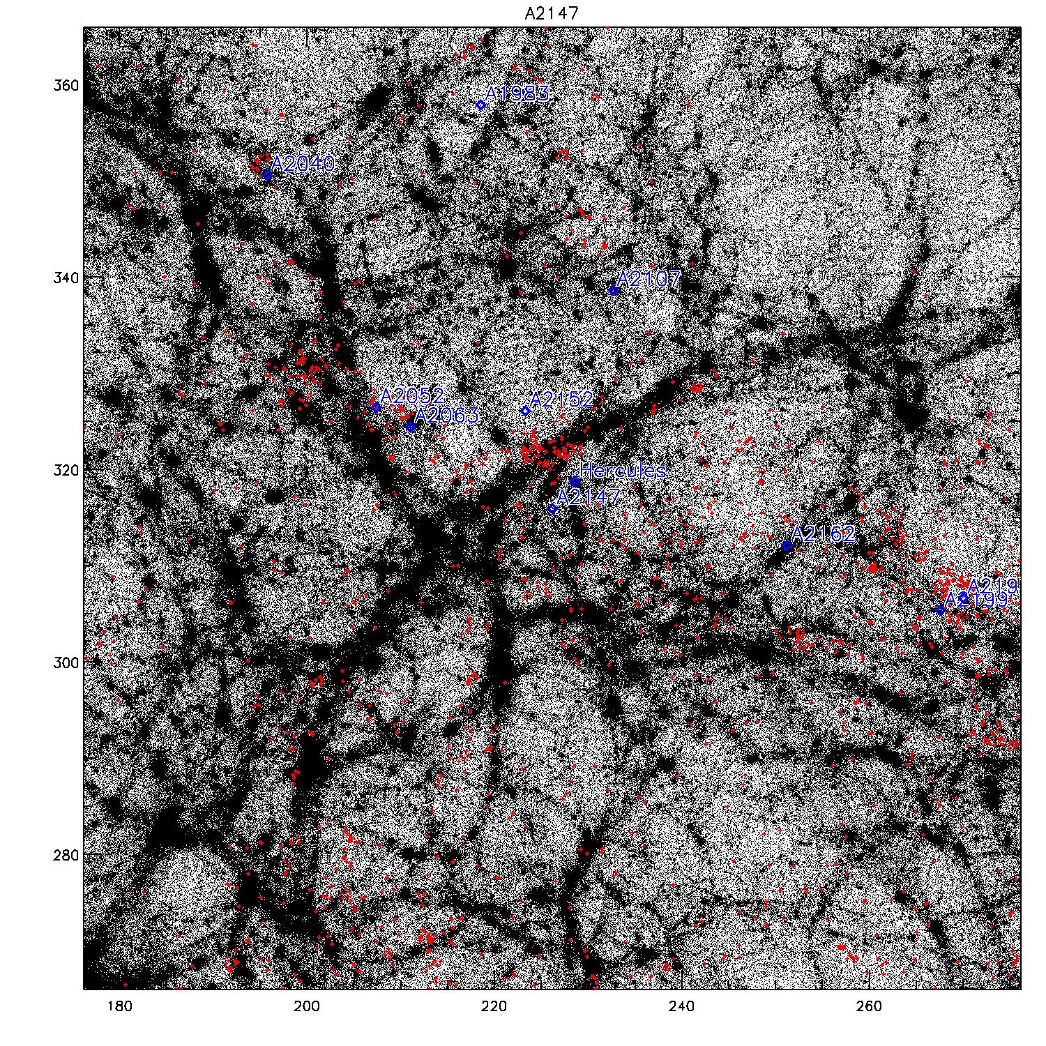
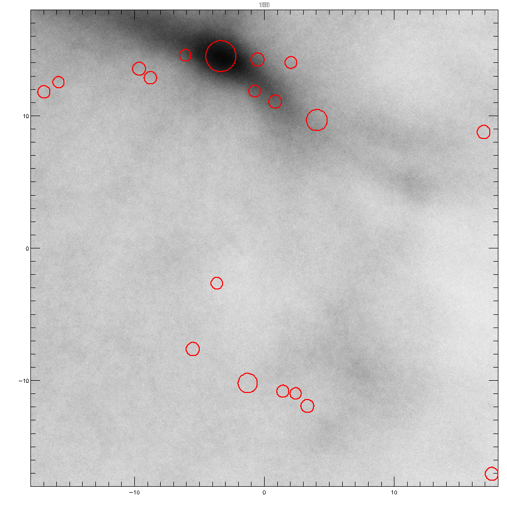
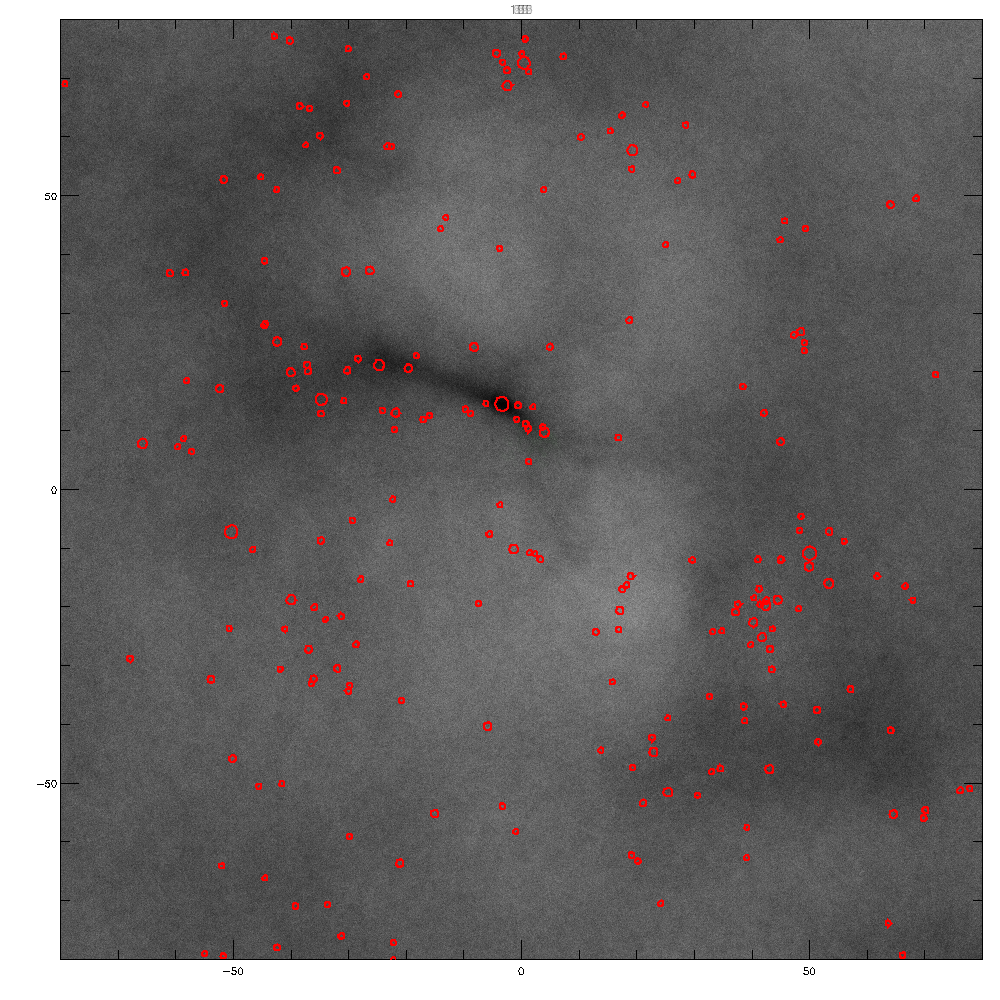
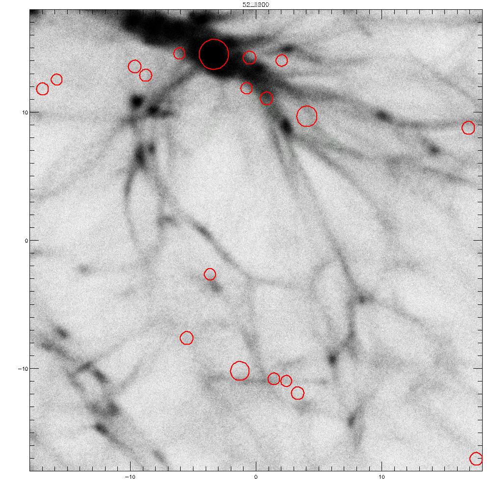
Individual comparions for all 200 realizations
Position of galaxies (applying a magnitude cut as before) for the 200 ralizations (left), for the
Mathis et al. 2002 simulation (middle) and for the 2MKS galaxy cataluge (right). Bluc circles mark
the size of clusters above 1.5e14 Msol. Shown is always a 50 Mpc cubic region.
Global density comparisons
Mean density as function of distance, using galaxies with m_k<11.25 from the different simulations compared to 2MKS.
Right panel: roughly renormalized at r=50-70 Mpc. Blue: based on Matthis 2002 (Klaus); Red: based on 52_2600 (Jenny);
Black: 2MKS.
Global radial veocity comparison
Hubble flow using galaxies with m_k<11.25 from the different simulations compared to observations.
Left panel: based on Mathis 2001 (Klaus). Right panel: based on 52_2600 (Jenny).
